Separate source memory from propagation and material memory

Begin with competing explanations

Suppose a detector shows a decaying signal after the source command goes low. Possible causes include a slow source, a traveling pulse still in the path, stored energy in a resonator, delayed material response, reflections, and detector filtering. Several can occur simultaneously. Naming the trace ringdown before testing these alternatives can build the conclusion into the analysis.

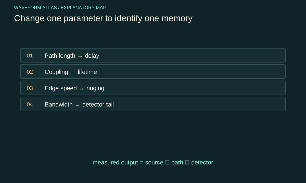
Write a short hypothesis table before collecting the main data. For each explanation, identify a parameter that should change its timing or shape. Path length changes propagation delay; coupling changes a resonator's escape rate; edge duration changes switching excitation; detector bandwidth changes instrumental response. The experiment need not exhaust every imaginable mechanism. It should discriminate the plausible mechanisms at the precision relevant to the claim. This preparation makes the later controls purposeful rather than a collection of unrelated checks.

Measure the local output, not just the command

A digital command is an instruction to the source, not a direct measurement of emitted power or applied force. Output stages, actuators, switches, and loads introduce delay and residual response. Place a monitor as close as practical to the system input and characterize its own bandwidth. The monitor establishes when the physical drive reaches the desired low level.

For an optical experiment, a calibrated pickoff can track incident light. For an electrical system, a suitable voltage or current measurement can track the delivered drive. For a mechanical system, the relevant quantity may be force rather than actuator command. The monitor should not significantly change the system being studied, or its loading must be included. A claim of free evolution is stronger when it includes a bound on residual drive relative to the decaying system signal, especially at late times.

Use distance to identify propagation

Repeat the measurement at several known path lengths while keeping the source and detector electronics as similar as possible. A direct nondispersive feature should shift by ΔL/v. Plotting measured arrival time against distance separates the slope, associated with propagation, from a fixed intercept containing trigger and electronics delays.

An illustrative acoustic increase of 1.715 meters predicts an extra 5 milliseconds at 343 meters per second. If the entire trace translates without much reshaping, a simple delay model may be adequate. If the tail broadens with distance, dispersion, scattering, or multiple paths may matter. Changing path length can also change alignment and collection efficiency, so power normalization should be monitored. A timing shift alone does not identify loss; it identifies a relation between source history and detector history under the chosen geometry.

Change coupling to test stored-energy leakage

For a resonator, alter an external coupling parameter without intentionally changing the internal material. In the simple model, the total energy-decay rate is the sum of internal and external rates. Increasing an output coupling should shorten the lifetime and increase the fraction of stored energy leaving through that port, subject to changes in preparation and mode matching.

Measure both the decay and the relevant output power when possible. If the lifetime changes but the initial stored energy also changes, compare normalized traces and integrated outputs with a model that includes loading. An external coupler can shift resonance frequency or excite additional modes, so verify that the same mode is being followed. This control distinguishes energy escape from continued source emission more directly than a single source-off trace. It also prevents internal absorption from being inferred solely from a loaded lifetime.

Vary the switching edge to expose transients

Repeat the shutdown with several fall times or smooth envelopes while holding the preceding steady state fixed. A transient excited by a sharp edge should often change with the edge spectrum. A genuine late-time free-decay rate of a linear mode should remain approximately unchanged once the transient and residual drive are negligible.

The distinction between transient amplitude and decay rate is useful. A slower edge may excite less ringing without changing the resonator's loss coefficient. A different switch phase may change the initial free oscillation without changing the same coefficient. Record the actual delivered waveform for each setting, because the hardware may not reproduce the command. If a claimed unusual decay appears only with one abrupt edge, investigate switching artifacts and parameter changes before proposing a new propagation or collapse mechanism.

Test the detector as a separate system

Measure or bound the detector impulse response, bandwidth, baseline recovery, and saturation threshold. A slow detector can produce a tail after the physical input has ended. A saturated detector can recover gradually and imitate a long decay. Digital filtering can add still another memory to the displayed signal.

Compare measurements at different bandwidth settings or with an independent detector whose response is faster than the suspected physical process. If the inferred lifetime tracks the instrument setting, the instrument is part of the explanation. Deconvolution can help only when the response is known and the relevant frequencies remain measurable above noise. Retain raw data and document any filtering. A visually smooth trace is not necessarily a more faithful trace, and aggressive smoothing can conceal short echoes, beating, or switching artifacts that would otherwise distinguish the mechanisms.

Separate amplitude, power, and phase observables

A source-off test should state what the detector measures. In a linear oscillator, amplitude and energy decay at different rates. In a quantum or coherent optical experiment, phase-sensitive amplitude, photon flux, population, and fringe visibility carry different information. A fading interference signal can reflect phase randomization even when energy remains.

Use complementary readouts when the claim depends on this distinction. Direct power detection and coherent amplitude detection can test the expected factor-of-two relation in a simple cavity. Population and phase measurements can separate relaxation from dephasing in a two-level model. A spatially resolved detector can distinguish mode redistribution from attenuation in one collection channel. The analysis should not silently replace one observable with another. State the measurement equation and its calibration before assigning the fitted slope to a physical lifetime.

Plan the fitting interval and uncertainty

A useful fit starts after the drive has ended at the system and after unmodeled fast transients have settled. It ends before background, detector noise, or another mode dominates beyond the model's validity. These choices should be justified by controls, not tuned solely to produce a straight semilog line.

Fit an explicit background where appropriate and inspect residuals. Repeat the fit across nearby intervals to assess stability. Report repeatability across separate acquisitions and systematic uncertainties from calibration, timing, and residual drive. If a single exponential fails, compare physically motivated alternatives such as two modes, nonlinear damping, or a convolution with detector response. Additional fit parameters do not automatically identify additional physical reservoirs. The data need enough duration and dynamic range to distinguish those models, and independent controls should constrain the interpretation.

Close a practical energy budget

When the question concerns disappearance of energy, integrate calibrated power over time and include the relevant ports. For a resonator, compare initial stored energy with emitted energy and inferred internal dissipation. For a traveling pulse, compare input and output pulse energies with sufficient aperture and duration to collect delayed components.

Suppose an illustrative system contains 100 microjoules at cutoff. Measurements find 60 microjoules in one output and 25 microjoules in another. The remaining 15 microjoules are not automatically heat; they may include unmeasured scattering, residual storage, calibration error, or true internal absorption. A thermal measurement or additional collection can constrain the remainder. State the unresolved budget explicitly. This does not weaken the experiment; it prevents a partially observed system from being described as if every energy channel had been measured.

State the conclusion at the level the controls support

A strong conclusion might identify a propagation delay, a loaded energy lifetime, a residual-drive upper bound, and a detector-corrected settling time. It can also state which competing models were inconsistent with the controlled changes. Those results are concrete and reproducible without claiming more than the data show.

If several explanations remain compatible, report that limitation and the next discriminating measurement. A source-off experiment does not by itself decide whether quantum mechanics needs an objective-collapse modification. Such a claim requires a specific alternative prediction that differs from ordinary source, propagation, and open-system dynamics. The practical success criterion is simpler: explain the observed ending using measured source behavior, known paths, calibrated response, and an explicit energy account. That framework makes even a complicated tail scientifically useful rather than merely surprising.

A preregistered timing convention is useful even for a small laboratory test: define the source threshold, detector threshold, and fit window before comparing configurations. Otherwise an analyst can unintentionally choose different parts of differently shaped traces and call the difference a changed propagation speed. Saving the full traces allows alternative estimators to be checked without replacing the original definition after seeing the outcome.

Store calibration records with those traces so later comparisons can distinguish a physical change from a changed gain, bandwidth, sampling rate, or detector alignment.

Go to the original work.

These links identify the sources behind specific claims. Verification scope varies by source and is stated below.

1. 1 / University teachingSignals and Systems — Alan V. Oppenheim, lecture notes ↗

   Alan V. Oppenheim. Signals and Systems — Alan V. Oppenheim, lecture notes. 2011.

   Convolution, linear systems, filtering and feedback

   Verification scope: Official course notes and topic records inspected

2. 2 / University teachingWave Propagation — Triantaphyllos Akylas, lecture notes ↗

   Triantaphyllos Akylas. Wave Propagation — Triantaphyllos Akylas, lecture notes. 2017.

   Transient wave propagation, elastic modes, interfaces and water waves

   Verification scope: Official chapter contents and author-written course records inspected

3. 3 / Primary researchCavity ring-down spectrometer for high-fidelity molecular absorption measurements ↗

   H. Lin; Z. D. Reed; V. T. Sironneau; J. T. Hodges. Journal of Quantitative Spectroscopy and Radiative Transfer 161, 11–20 (2015).

   DOI: 10.1016/j.jqsrt.2015.03.026

   Exponential cavity decay fitting, baseline offsets and a loss budget separating mirror loss, etaloning, scattering and absorption.

   Verification scope: NIST-hosted full text: title page and relevant decay-fit/loss-budget passages inspected; not every section reread.

4. 4 / University teachingElectromagnetics and Applications — lecture notes ↗

   David H. Staelin. Electromagnetics and Applications — lecture notes. 2009.

   Poynting theorem, boundary conditions, material response and polarization

   Verification scope: Official author-written course and topic records inspected

5. 5 / University teachingElectromagnetics and Applications: Lecture 19, Electromagnetic Radiation ↗

   Electromagnetics and Applications: Lecture 19, Electromagnetic Radiation.

   Retarded electromagnetic propagation and radiated fields

   Verification scope: Official author-written lecture description inspected

6. 6 / University teachingFundamentals of Photonics: Quantum Electronics — lecture notes ↗

   Franz X. Kärtner. Fundamentals of Photonics: Quantum Electronics — lecture notes. 2006.

   Population dynamics, absorption/gain, Rabi oscillations and coupled modes

   Verification scope: Official author-written course materials and topic mapping inspected

7. 7 / University teachingLecture 16: Fourier transform — Signals and Systems ↗

   Lecture 16: Fourier transform — Signals and Systems.

   Finite pulse Fourier transforms and time/frequency scaling

   Verification scope: Official lecture equations inspected

8. 8 / University teachingDamped Oscillations — University Physics Volume 1 ↗

   OpenStax. University Physics Volume 1, Section 15.5: Damped Oscillations.

   Linear viscous damping and damping regimes

   Verification scope: Official textbook section and equation record inspected

9. 9 / University teachingQuantum Optical Communication — Jeffrey H. Shapiro, readings and lecture slides ↗

   Jeffrey H. Shapiro. Quantum Optical Communication — Jeffrey H. Shapiro, readings and lecture slides. 2016.

   Author-written quantum attenuator, amplifier, detection and parametric interaction framework

   Verification scope: Official course materials and topic mapping inspected

10. 10 / Primary researchCoupled-cavity ring-down spectroscopy technique ↗

    J. B. Courtois; J. T. Hodges. Optics Letters 37(16), 3354–3356 (2012).

    DOI: 10.1364/OL.37.003354

    Controlled optical feedback changes a coupled cavity decay; reported ring-down time increases from 210 to 280 microseconds.

    Verification scope: NIST abstract and primary PDF bibliographic page inspected

11. 11 / University teachingElectromagnetics and Applications, Chapter 9: Electromagnetic Waves ↗

    David H. Staelin. Electromagnetics and Applications, Chapter 9: Electromagnetic Waves. 2009.

    Planar boundaries, complex media, waveguides and cavity resonators; §9.4 defines Q through energy loss and exponential decay.

    Verification scope: Current official PDF download verified; relevant chapter passages inspected, not an entire textbook reread.