Stored energy after the drive ends

The initial condition supplies the motion

Before shutdown, a drive continually exchanges energy with the resonator. At the moment the drive ends, the system generally retains a displacement, velocity, field, or other stored excitation. Those initial conditions determine the free evolution. A mass on a spring does not need continuing external force to keep moving; its kinetic and potential energies exchange while damping removes energy from the chosen mode.

The same logic applies to an electromagnetic cavity, although the stored energy resides in electric and magnetic fields. The source-off event changes the forcing term, not the entire state. A ringdown experiment therefore prepares a state and observes its subsequent relaxation. The preparation phase matters because switching at different phases can leave different amplitudes or combinations of modes. Comparing decay curves without checking the initial condition can confuse a changed excitation pattern with a changed loss mechanism.

A linear oscillator gives the basic solution

For m ẍ + b ẋ + kx = 0, define ω0 = √(k/m) and γ = b/(2m). In the underdamped regime γ < ω0, the displacement is exp(−γt)[A cos(ωdt)+B sin(ωdt)], with ωd = √(ω0²−γ²). The constants A and B follow from initial displacement and velocity. The oscillation frequency is slightly below the undamped natural frequency.

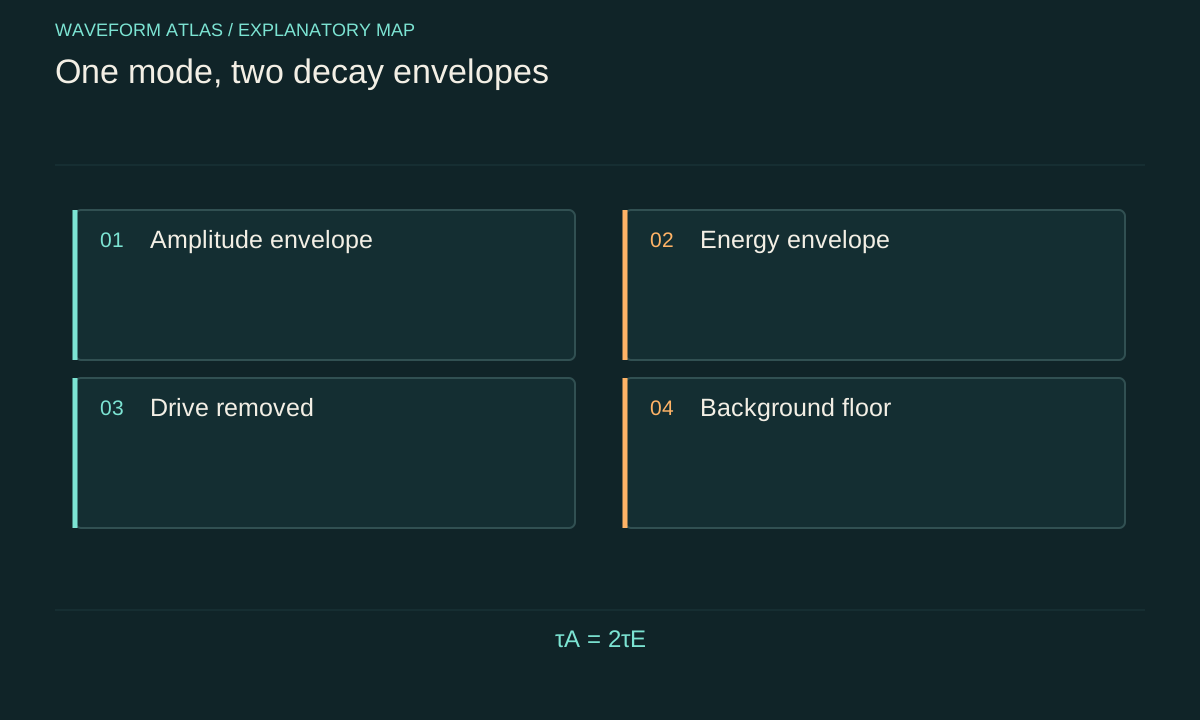
The envelope decay time is τA = 1/γ. In weak damping, cycle-averaged energy decays approximately as exp(−2γt), giving τE = 1/(2γ). Exact instantaneous mechanical energy can have small within-cycle structure because dissipation depends on velocity, but its derivative is unambiguously dE/dt = −b ẋ². These equations make the energy destination explicit: the damping term transfers mechanical energy to degrees of freedom omitted from the ideal oscillator coordinate.

The detector determines which lifetime appears

A displacement sensor may report the oscillatory amplitude directly, while a power or intensity detector reports a quantity quadratic in field amplitude. If an amplitude envelope falls to 1/e in one second, the associated energy envelope falls to 1/e in about half a second in the simple model. Confusing these observables produces a factor-of-two error in decay rates and quality factors.

An optical heterodyne measurement can access field quadratures, whereas a direct intensity measurement generally follows photon flux or power. The two records can legitimately show different exponential slopes. A detector voltage is not automatically an amplitude measurement merely because it is called a signal. Calibration and the detector's physical response determine the relation. Before fitting, state the model connecting the recorded voltage or counts to the resonator variable, including offsets, saturation, and finite instrument response.

Independent escape rates add in a simple model

Let a cavity's stored energy satisfy dU/dt = −κU. If independent memoryless channels remove fractions of the same stored energy, κ can be written as κ1+κ2+κinternal. The total energy lifetime is 1/κ. The portion ultimately escaping through channel j is κj/κ times the initial stored energy when the rates remain constant and no drive returns energy.

For an illustrative cavity with rates 2, 1, and 1 inverse seconds, the total lifetime is 0.25 second. Half the initial energy exits the first port, one quarter exits the second, and one quarter is internally dissipated. A measured ringdown alone gives the total rate of 4 inverse seconds, not that partition. Port-resolved measurements or controlled changes in coupling are needed to infer individual contributions. The additive model can fail when channels interfere coherently or retain significant memory.

Several modes can imitate unusual decay

If two nearby modes are excited, their fields add before an amplitude-sensitive measurement and can produce beating. The measured intensity can then oscillate under an overall decaying envelope. A fit to one exponential may assign different decay times depending on which segment is selected. This does not necessarily mean the damping law changes with time.

A frequency-domain measurement can reveal nearby resonances, while changing the excitation geometry can favor one mode over another. Spatially resolved detection also helps because distinct modes have different shapes. If the detector sums incoherent power from several modes, the trace may instead be a sum of exponentials without visible beating. Both cases require more information than one fitted lifetime. Adding several exponential terms can improve a numerical fit, but physical identification of the terms needs independent evidence such as mode frequencies, spatial patterns, or controlled coupling changes.

Nonlinear loss changes the envelope

Viscous damping produces an exponential envelope only within its linear regime. Dry friction can produce a roughly linear decrease in oscillation amplitude over successive cycles. A loss force proportional to a higher power of velocity can make the decay rate depend on amplitude. Optical absorption can also change as a material heats or saturates, causing the later ringdown to differ from the earlier portion.

Repeat the experiment across several initial energies. If normalized curves fail to overlap, a constant-rate model may be inadequate. Check detector linearity before assigning the difference to the resonator. Plotting instantaneous decay rate, where noise permits, can reveal systematic amplitude dependence. A physically motivated nonlinear model should predict how the curve changes with preparation, temperature, or geometry. Merely labeling a nonexponential trace anomalous does not identify a new mechanism; ordinary nonlinearities often provide testable explanations.

Residual driving must be bounded

A source may have finite extinction, and a switch can leak a small continuing field. Near the end of a ringdown, that residual drive can become comparable to the decaying field. Coherent interference between the residual input and stored field can distort the trace, while incoherent background can create an apparent floor. The result can look like a very long lifetime if the background is omitted.

Monitor the source at the resonator input, vary switch extinction or drive detuning, and compare the inferred decay across those changes. A background measurement with the resonator unexcited helps characterize the detector offset but may not capture coherent leakage. The useful fit interval begins after the switching transient and ends before unmodeled backgrounds dominate. Reporting that interval and the residual-drive bound makes the lifetime interpretable. A control command alone is not evidence that the physical forcing has reached zero.

Ringdown and linewidth should be compared carefully

For a narrow, isolated linear resonance with energy-decay rate κ in radians-per-second-compatible units, the angular-frequency power linewidth is κ and Q ≈ ω0/κ. Thus an energy lifetime τE gives Q ≈ ω0τE. A resonance at 100 kilohertz with τE = 1 millisecond has an illustrative Q of about 628 and a linewidth near 159 hertz.

A swept response can be broader than this prediction if the resonance frequency drifts or fluctuates during the measurement. Ringdown can also be affected by phase noise depending on how amplitude is extracted. Differences between methods therefore reveal something about the apparatus rather than automatically invalidating either method. State whether linewidth means full width at half maximum of power, amplitude, or another quantity. The simple lifetime-linewidth relation rests on a specific single-mode response model and should not be extended indiscriminately to strongly damped or nonstationary systems.

Extracting a decay time without hiding the evidence

Fit the recorded observable with an explicit background and appropriate noise model. Inspect residuals and test stability against changing the fit start and end times. Repeated acquisitions reveal variability that one least-squares covariance estimate may miss. If photon counts are small, count statistics matter; if an analog detector has correlated noise, treating every sample as independent can understate uncertainty.

NIST's cavity ringdown work illustrates that high-fidelity absorption measurements require attention to baseline, optical feedback, and other instrument effects. The general lesson is that a straight-looking semilog plot is only a diagnostic. A slightly incorrect baseline can bend the late-time trace or produce a false slope. Preserve the original units and show the fitted model against the data. A credible lifetime comes with enough information to understand which physical and instrumental assumptions made it measurable.

What ringdown says about disappearance

Ringdown establishes how a selected excitation relaxes after preparation. A shorter lifetime means faster energy escape from that mode under the measurement conditions. It does not identify whether the energy became heat, emerged as radiation, entered a support, or transferred into another mode unless those channels are separately constrained.

In a quantum description, a cavity field can decay through coupling to outside modes, and conditional detection records can carry information about individual emissions. That description is compatible with ordinary unitary dynamics of a larger system and an open-system description of the cavity. The decay is not, by itself, evidence for objective reduction of the universal state. Keeping the subsystem boundary explicit lets ringdown remain a precise and powerful measurement: it quantifies stored-energy lifetime while leaving broader claims to experiments designed to distinguish them.

A useful final control repeats the decay with the detector moved to another point on the same mode. The inferred lifetime should agree after accounting for the different signal amplitude. A changed lifetime can reveal mode mixing, position-dependent background, or a measurement that was not tracking one isolated mode.

Go to the original work.

These links identify the sources behind specific claims. Verification scope varies by source and is stated below.

1. 1 / University teachingDamped Oscillations — University Physics Volume 1 ↗

   OpenStax. University Physics Volume 1, Section 15.5: Damped Oscillations.

   Linear viscous damping and damping regimes

   Verification scope: Official textbook section and equation record inspected

2. 2 / University teachingFundamentals of Photonics: Quantum Electronics — lecture notes ↗

   Franz X. Kärtner. Fundamentals of Photonics: Quantum Electronics — lecture notes. 2006.

   Population dynamics, absorption/gain, Rabi oscillations and coupled modes

   Verification scope: Official author-written course materials and topic mapping inspected

3. 3 / University teachingOscillations: Key Equations — University Physics Volume 1 ↗

   Oscillations: Key Equations — University Physics Volume 1.

   Oscillator equations and amplitude/frequency conventions

   Verification scope: Official equation page inspected

4. 4 / Primary researchCavity ring-down spectrometer for high-fidelity molecular absorption measurements ↗

   H. Lin; Z. D. Reed; V. T. Sironneau; J. T. Hodges. Journal of Quantitative Spectroscopy and Radiative Transfer 161, 11–20 (2015).

   DOI: 10.1016/j.jqsrt.2015.03.026

   Exponential cavity decay fitting, baseline offsets and a loss budget separating mirror loss, etaloning, scattering and absorption.

   Verification scope: NIST-hosted full text: title page and relevant decay-fit/loss-budget passages inspected; not every section reread.

5. 5 / University teachingQuantum Optical Communication — Jeffrey H. Shapiro, readings and lecture slides ↗

   Jeffrey H. Shapiro. Quantum Optical Communication — Jeffrey H. Shapiro, readings and lecture slides. 2016.

   Author-written quantum attenuator, amplifier, detection and parametric interaction framework

   Verification scope: Official course materials and topic mapping inspected

6. 6 / University teachingWave Propagation — Triantaphyllos Akylas, lecture notes ↗

   Triantaphyllos Akylas. Wave Propagation — Triantaphyllos Akylas, lecture notes. 2017.

   Transient wave propagation, elastic modes, interfaces and water waves

   Verification scope: Official chapter contents and author-written course records inspected

7. 7 / University teachingSignals and Systems — Alan V. Oppenheim, lecture notes ↗

   Alan V. Oppenheim. Signals and Systems — Alan V. Oppenheim, lecture notes. 2011.

   Convolution, linear systems, filtering and feedback

   Verification scope: Official course notes and topic records inspected

8. 8 / Primary researchCoupled-cavity ring-down spectroscopy technique ↗

   J. B. Courtois; J. T. Hodges. Optics Letters 37(16), 3354–3356 (2012).

   DOI: 10.1364/OL.37.003354

   Controlled optical feedback changes a coupled cavity decay; reported ring-down time increases from 210 to 280 microseconds.

   Verification scope: NIST abstract and primary PDF bibliographic page inspected

9. 9 / University teachingElectromagnetics and Applications, Chapter 9: Electromagnetic Waves ↗

   David H. Staelin. Electromagnetics and Applications, Chapter 9: Electromagnetic Waves. 2009.

   Planar boundaries, complex media, waveguides and cavity resonators; §9.4 defines Q through energy loss and exponential decay.

   Verification scope: Current official PDF download verified; relevant chapter passages inspected, not an entire textbook reread.

10. 10 / University teachingFundamentals of Photonics, Chapter 2: Classical Electromagnetism and Optics ↗

    Franz X. Kärtner. Fundamentals of Photonics, Chapter 2: Classical Electromagnetism and Optics. 2006.

    §§2.1.6–2.1.8: group velocity, Gaussian broadening and complex index; §§2.2.1–2.2.5: boundary phase matching, flux coefficients and total internal reflection; §2.3: multilayers.

    Verification scope: Relevant PDF passages inspected; uses exp(+jωt), opposite to the article’s exp(−iωt) loss-sign convention.

11. 11 / University teachingStructural Motion Engineering ↗

    J. J. Connor; S. Laflamme. Structural Motion Engineering. 2014. doi:10.1007/978-3-319-06281-5.

    DOI: 10.1007/978-3-319-06281-5

    Author-hosted fourth draft, §4 Coulomb damping: force of fixed magnitude and work per cycle W = 4FcA; printed edition published by Springer.

    Verification scope: Publisher metadata and indexed author-hosted draft passage for Eqs. (4.7)–(4.8) inspected. Whole PDF could not be loaded because of tool size limit.