Removing a quantum drive

The state at switch-off remains the starting point

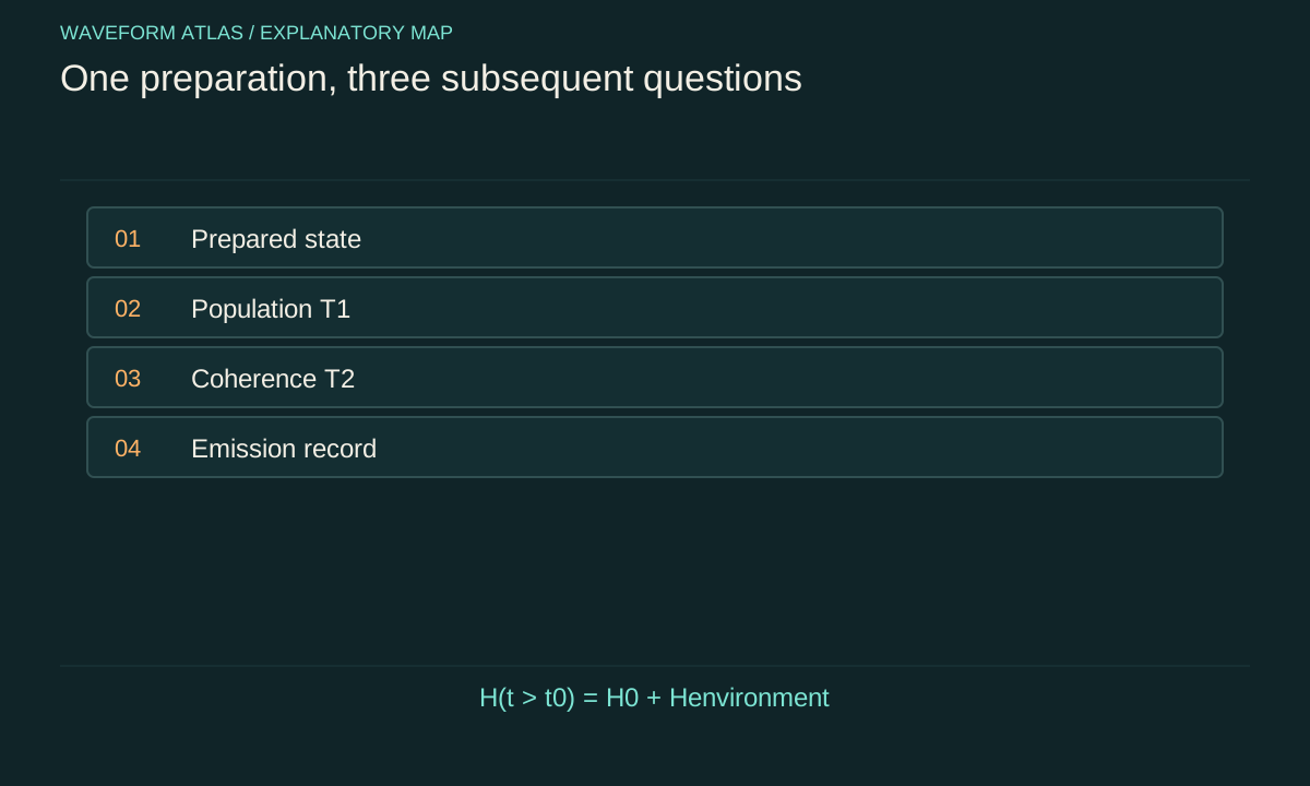
A driven quantum system can be described by a Hamiltonian H(t) = H0+Hdrive(t), possibly with additional environmental coupling. Setting the drive term to zero leaves the state at that instant as the initial condition for later evolution. The state does not automatically reset because the term that prepared it has disappeared.

For a two-level system, a pulse can leave a ground state, an excited state, or a superposition depending on pulse area, phase, detuning, and imperfections. For an oscillator, the drive can leave a coherent displacement or a more complicated state. Subsequent behavior depends on H0 and the environment. A source-off experiment should therefore specify both the switching operation and the prepared state. Without that information, a later population or field trace cannot be uniquely interpreted as evidence about the effect of turning off the drive itself.

An ideal two-level pulse gives a concrete example

In an ideal resonantly driven two-level system with constant Rabi frequency Ω and an appropriate phase convention, a pulse of duration t produces a rotation whose angle is Ωt. Starting in the ground state, the excited-state probability is sin²(Ωt/2). A π pulse ideally prepares the excited state, while a π/2 pulse prepares an equal-population superposition with a phase set by the drive.

If Ω/(2π) is 1 megahertz, the ideal π-pulse duration is 0.5 microsecond and the π/2-pulse duration is 0.25 microsecond. Removing the drive after either duration leaves different states. These are calculated examples under the rotating-wave and coherent-control assumptions, not universal pulse recipes. Detuning, finite bandwidth, additional levels, and relaxation during the pulse alter the result. Measuring only that the source has turned off does not establish which state was prepared.

Free evolution can change phase without changing populations

For an isolated two-level system with energy separation ℏω0, a superposition acquires a relative phase at rate ω0 under the free Hamiltonian. The populations in the energy basis remain constant. A later phase-sensitive measurement can reveal the accumulated phase even though a direct energy measurement would show no population change.

This is why the measurement basis matters. A state that appears unchanged to one detector can produce an oscillating signal in another basis. A Ramsey-type sequence uses a second controlled pulse to convert relative phase into a population difference. Removing the first drive is part of the preparation sequence, not a measurement in itself. The distinction also prevents a common confusion between absence of a visible oscillation in one observable and absence of coherent quantum evolution. The complete state can evolve while a selected expectation value remains fixed.

Relaxation needs an energy-transfer channel

An excited system coupled to electromagnetic or material modes can transfer energy to them. In a simple Markovian model, excited-state population decays exponentially with a lifetime T1. The emitted energy can appear as a photon, phonon, or another excitation depending on the system and coupling. The source need not remain on for that later emission to occur.

For an illustrative initial excited population of one and T1 = 10 microseconds, the population after 10 microseconds is 1/e, about 0.368. The lost population is not a direct calorimetric measurement, but under the specified two-level decay model it corresponds to excitation transferred out of the system. Additional levels, thermal re-excitation, nonradiative channels, and detector inefficiency complicate that inference. A lifetime measurement should identify the measured population or emission signal and distinguish it from the coherent field amplitude.

Dephasing can occur without the same energy change

Environmental fluctuations can randomize relative phase while leaving energy-basis populations approximately unchanged. In a commonly used Markovian two-level model, 1/T2 = 1/(2T1)+1/Tφ, where T2 is coherence decay and Tφ is pure-dephasing time. The equation is model-specific and does not say every system has one universal dephasing rate.

A source-off population trace measures different information from an interference contrast or phase-sensitive trace. For example, a state can retain equal ground and excited populations while its off-diagonal density-matrix element becomes small. Conversely, energy relaxation changes both population and coherence under the amplitude-damping model. Measuring both quantities tests whether a proposed environmental account is consistent. A disappearance of coherent signal after drive removal is therefore not enough to conclude that all excitation has left the system, let alone that a fundamental collapse law has acted.

A cavity illustrates stored quantum excitation

A driven cavity can contain an optical state when its input is removed. Under linear coupling to an external vacuum field, the intracavity amplitude decays while energy leaks into outgoing modes. A coherent state remains coherent in the ideal attenuator model with a reduced amplitude, even though its mean photon number falls. Other input states can develop different reduced-state properties under the same loss channel.

This example separates energy loss from an automatic loss of every form of coherence. The combined cavity and outgoing field retain a larger dynamical account, while an observer who traces out the outgoing modes sees an open-system evolution. The external light can be detected later, carrying energy and information about the initial state. Turning off the laser is not what destroys the photon energy; the cavity's coupling determines how it is released after the preparation ends.

A detection record changes the conditional description

If emitted photons are monitored, the observer can update a conditional state using the measurement record. A detected event and a no-detection interval can carry different information. Averaging over all possible records gives an unconditional evolution that can be written as an open-system master equation under suitable approximations.

These descriptions should not be conflated. A conditional jump in a mathematical state estimate is tied to a specified measurement scheme, efficiency, and record. An unmonitored system can be described without assigning the same observed sequence. Neither formulation alone establishes an objective-collapse mechanism acting independently of measurement context. A source-off experiment must say whether its claim concerns a measured event, an ensemble population, a conditional trajectory, or a fundamental law. The same raw photon-count data can support ordinary decay physics without deciding every interpretive question about quantum measurement.

The switch can perturb the quantum system

A physical drive cutoff has finite duration and can change more than its intended amplitude. Frequency chirp, phase transients, leakage, and changes in nearby fields can perturb the prepared state. If the drive also modifies a resonance or coupling, removing it changes H0 effectively as well as Hdrive. A sudden parameter change can produce dynamics different from a clean end to resonant forcing.

Characterize the delivered pulse at the system, not only the command waveform. Vary the cutoff shape and compare the resulting state or decay trace. A control experiment with the same switching electronics but no intended excitation can reveal pickup or background. These checks are especially important when a small post-pulse signal is attributed to unusual quantum behavior. Ordinary control imperfections can be coherent and reproducible, so repeatability alone does not rule them out.

Design measurements that separate the alternatives

A useful sequence prepares a state, removes the drive, waits a controlled delay, and measures one of several observables. Population measurements estimate relaxation. Phase-sensitive sequences estimate coherence. Time-resolved emission measures an output channel. Repeating with different preparation phases and amplitudes helps test the control model.

Detector response and pulse leakage should be calibrated independently. If the measured field decays twice as slowly as intensity, that can be the expected amplitude-energy relation rather than a discrepancy. If coherence decays faster than population permits in the chosen model, an additional dephasing channel or technical phase noise may be needed. If output counts do not match population loss, unobserved channels and detection efficiency must be considered. The aim is a joint account of several observables, because any one trace leaves important alternatives unresolved.

What a successful source-off experiment establishes

A successful experiment identifies the prepared state to the required accuracy, bounds residual forcing, and measures subsequent evolution under known conditions. It can determine lifetimes, coupling rates, phase stability, or emitted temporal modes. Those are substantial results even when no claim is made about fundamental collapse.

The source-off boundary is useful because it separates preparation from observation, but the separation is never purely verbal. It must be supported by timing, calibration, and a model of the remaining couplings. The state then follows the dynamics that remain, whether approximately isolated, dissipative, or actively controlled. Keeping drive removal distinct from relaxation and measurement avoids a false narrative in which a quantum system stops existing or becomes classical merely because the external oscillator or laser that prepared it has been switched off.

Thermal occupation adds a further distinction. If the environment can re-excite the system, its long-time population need not be the ground state. Upward and downward transition rates determine the stationary balance. A nonzero late-time population can then be ordinary thermal equilibrium rather than evidence of residual coherent driving; temperature and phase-sensitive controls help separate those possibilities.

Go to the original work.

These links identify the sources behind specific claims. Verification scope varies by source and is stated below.

1. 1 / University teachingQuantum Optical Communication — Jeffrey H. Shapiro, readings and lecture slides ↗

   Author-written quantum attenuator, amplifier, detection and parametric interaction framework

   Verification scope: Official course materials and topic mapping inspected

2. 2 / University teachingFundamentals of Photonics: Quantum Electronics — lecture notes ↗

   Population dynamics, absorption/gain, Rabi oscillations and coupled modes

   Verification scope: Official author-written course materials and topic mapping inspected

3. 3 / University teachingSignals and Systems — Alan V. Oppenheim, lecture notes ↗

   Convolution, linear systems, filtering and feedback

   Verification scope: Official course notes and topic records inspected

4. 4 / Primary experimentCavity ring-down spectrometer for high-fidelity molecular absorption measurements ↗

   Intensity ringdown fits and distinction between absorption and baseline loss

   Verification scope: Author-hosted paper's measurement model and discussion excerpts inspected