Why some frequencies produce a stronger response

Name the response that becomes large

A vibrating mass, an electrical circuit, an optical cavity and a quantum transition can all show resonant behavior. Their common feature is a frequency-selective response associated with the system's dynamics. The measured quantity might be displacement, current, transmitted power or transition probability. A statement that a system resonates is incomplete until that observable and the driving conditions are specified.

The largest raw output is not automatically the system's resonance. A source may itself emit more strongly at one frequency, or a detector may be more sensitive there. A calibrated response compares output with the actual input and includes phase where possible. This separates a property of the system from a feature introduced by the excitation or measurement chain.

A simple oscillator supplies the baseline

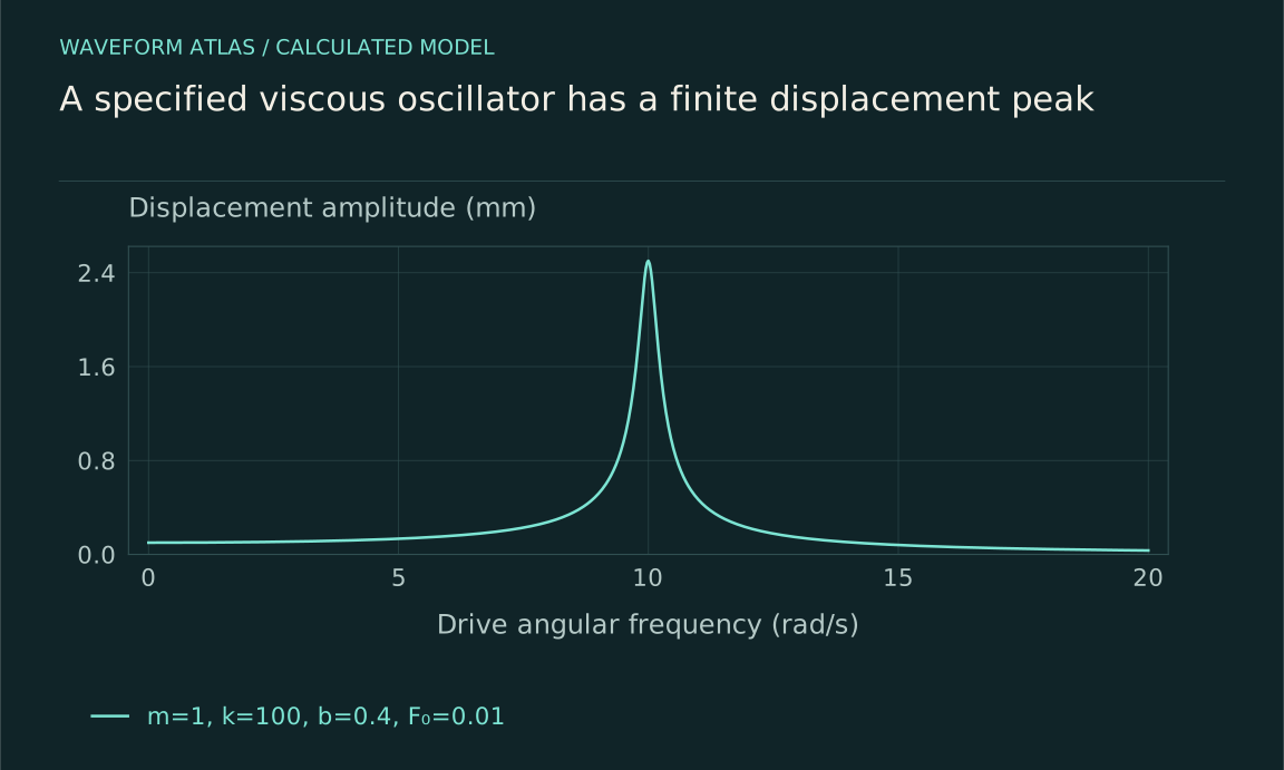
Consider m ẍ+b ẋ+kx=F₀cosωt, with positive mass, damping and stiffness. The undamped natural angular frequency is ω₀=√(k/m). In steady state, the displacement amplitude is A=F₀/√[(k−mω²)²+(bω)²]. At low frequency the spring stiffness dominates; at high frequency inertia dominates. Between them, their opposing contributions can nearly balance, making the response larger.

This equation is a model of linear restoring force and viscous damping. It does not describe every resonator exactly, but its parameters and assumptions are explicit. A measured response can be compared with it and deviations investigated. Large response is therefore a calculable dynamical effect, not a general rule that matching any two frequencies must produce unlimited motion.

Phase explains the energy transfer

Write x(t)=Acos(ωt−δ), where δ=atan2(bω,k−mω²). At low frequency displacement is nearly in phase with force. Near ω₀ it lags by approximately a quarter cycle, and at high frequency it approaches a half-cycle lag. The velocity phase determines the instantaneous work rate F(t)ẋ(t).

Averaging over a cycle gives input power equal to bω²A²/2 in steady state. The drive supplies exactly the energy dissipated by viscous damping. The phase relationship makes that positive average work possible. A large displacement without a specified force phase does not fully describe the energy exchange, which is why a complex transfer-function measurement is more informative than an amplitude-only curve.

Different observables can peak differently

Define β=b/(2m). The displacement amplitude has a positive-frequency maximum at ωr=√(ω₀²−2β²) when the expression is real and the damping is sufficiently small. It is therefore slightly below ω₀ at finite damping. In the same fixed-force viscous model, velocity amplitude and average dissipated power peak at ω₀. The word resonance can refer to these different conventions in different contexts.

A heavily damped system may have no distinct displacement peak at a nonzero frequency, even though the same differential equation remains valid. Quoting one universal resonant frequency without specifying the observable can then be misleading. The complete response function identifies what is enhanced, how sharply, and whether a peak is meaningfully resolved in the measured range.

Damping sets a tradeoff

Weak damping allows energy to remain in the system for many cycles. It can produce a large narrow response and a long decay after the drive is removed. Stronger damping reduces buildup and broadens the response, often making the system settle faster. These are related consequences of the same loss mechanism in a simple resonator model.

For weak damping, Q≈ω₀/(2β), and the near-resonant half-power bandwidth is approximately 2β in angular frequency. The amplitude ringdown envelope is approximately exp(−βt), while energy decays with twice that exponent. State which quantity is plotted and which width convention is used. Half-amplitude width is not half-power width, and confusing them creates incorrect numerical relationships among Q, linewidth and lifetime.

A numerical oscillator makes the scale concrete

Take m=1 kilogram, k=100 newtons per metre, b=0.4 newton-seconds per metre, and force amplitude F₀=0.01 newtons. Then ω₀=10 radians per second, β=0.2 per second and Q≈25. The quasistatic displacement is F₀/k=0.1 millimetres, while the displacement at ω₀ is F₀/(bω₀)=2.5 millimetres.

The approximate half-power bandwidth is 0.4 radians per second, and the amplitude envelope decays on a five-second scale after driving stops. These are calculated properties of an ideal linear model, not measured performance of a particular spring. A real spring must remain in its linear range, and the mounting, actuator and sensor can add modes or damping that the one-coordinate model omits.

Finite duration prevents instant steady buildup

The steady-state formula describes behavior after transients have decayed. A resonator switched on from rest takes time to build its stored energy. Sweeping frequency too quickly can produce a curve that differs from the steady response because the system still remembers earlier drive conditions. High-Q systems require especially careful timing because their memory is long.

In the ideal undamped model driven exactly at ω₀, the resonant solution can grow linearly in amplitude with time. That mathematical result assumes zero damping, exact tuning and indefinite validity of the linear model. Real systems add finite duration, detuning, nonlinear stiffness, saturation or damage. The ideal growth law is useful for understanding the limit, but it is not a prediction that every resonant experiment must diverge or destroy itself.

Quantum resonances require their own observable

A driven two-level quantum system responds strongly when the drive frequency is near its transition frequency. Under a specified coherent-drive approximation, populations can oscillate between levels, with detuning reducing the maximum transfer. Relaxation and dephasing alter the response and can produce a steady spectral line. This is related to frequency matching but is not identical to a classical displacement resonance.

Specify whether the measurement concerns transition probability after a pulse, steady absorption, fluorescence or another observable. Pulse duration and drive strength can set widths in addition to intrinsic decoherence. A resonance peak does not by itself show a collapse mechanism; it shows a frequency-dependent response that must be interpreted using the system's Hamiltonian, dissipation and measurement protocol.

Coupling and nonlinearity add structure

Two interacting resonators can have collective modes with different frequencies and shapes. A drive may couple strongly to one mode and weakly to another, so the number of visible peaks need not equal the number of degrees of freedom. Changing a tuning parameter can reveal hybridization or an avoided crossing. Damping and detector placement determine whether the features are resolved.

Nonlinear stiffness can make frequency depend on amplitude, bend response curves and create multiple stable driven responses in some regimes. Parametric modulation can supply energy by changing a system parameter rather than applying an additive force. These effects require more detailed models. They are reasons to investigate a deviation from the simple oscillator, not reasons to abandon energy accounting or label every large motion the same kind of resonance.

A missing peak can also result from symmetry. If a drive pushes two identical coupled masses equally, it preferentially excites their in-phase mode and may not excite an antisymmetric mode at all. A sensor measuring their sum can be insensitive to that antisymmetric motion even if another drive excites it. The system's modes exist independently of whether one chosen input-output channel displays them strongly.

This is why resonance identification often benefits from changing actuator or sensor position. A feature that appears in another channel can reveal a previously hidden mode, while a feature that follows the source rather than the sample suggests an excitation artifact. The number and height of peaks in one spectrum are therefore properties of the whole measurement arrangement as well as of the underlying dynamical system.

Establish resonance with complementary measurements

Measure the actual input, output amplitude and phase across frequency, then compare with the decay after a drive change. Vary drive strength to test linearity and repeat sweeps slowly enough to identify transient effects. A consistent model of frequency response and ringdown provides stronger evidence for a resonant mode than a single output maximum.

The resulting conclusion can be specific: this observable is enhanced near this mode under these coupling and loss conditions. That statement explains useful sensitivity and bandwidth tradeoffs while leaving room for additional modes or nonlinearities when measured. Resonance is a structured response to energy supplied by a drive, not a universal route to infinite amplitude, synchronization, wavefunction collapse or energy creation.

A calibrated sweep can use a reference force sensor so that the plotted quantity is displacement divided by applied force, rather than displacement divided by a generator voltage. The actuator's force per volt may vary strongly with frequency. Correcting that variation can remove an apparent peak or reveal a resonance that the source spectrum had hidden. The same logic applies to optical input power and electrical excitation current.

Phase data provide a second check because a resonant transfer function predicts a characteristic change across the response region. A source-amplitude bump alone need not produce that phase evolution in the sample. Neither signature is infallible in isolation, but their agreement with a time-domain decay and a consistent parameter model makes the inference substantially stronger.

Go to the original work.

These links identify the sources behind specific claims. Verification scope varies by source and is stated below.

1. 1 / University teachingOpenStax: Forced Oscillations ↗

   OpenStax: Forced Oscillations. https://openstax.org/books/university-physics-volume-1/pages/15-6-forced-oscillations

   A driven oscillator balances forcing, inertia, stiffness and damping.

   Verification scope: University textbook section inspected. This article derives exact peak and half-power conventions rather than adopting the section’s simplified peak and width wording.

2. 2 / University teachingFrequency response: Resonance, Bandwidth, Q factor ↗

   M. Chaniotakis and D. Cory (2006). Frequency response: Resonance, Bandwidth, Q factor. MIT OpenCourseWare 6.071J/22.071, Spring 2006.

   Quality factor, stored energy and half-power bandwidth for a specified circuit model.

   Verification scope: Visible first-page title and equations (1.11)–(1.18) inspected. The PDF metadata title differs; the document itself covers resonance, bandwidth and Q for RLC circuits.

3. 3 / University teachingInteraction of Light and Matter, Chapter 6 ↗

   F. Kärtner (2006). Interaction of Light and Matter, Chapter 6. MIT OpenCourseWare 6.974, Spring 2006.

   The course includes two-level dynamics, Rabi oscillations, density matrices, and energy/phase relaxation.

   Verification scope: Direct MIT chapter PDF passages on the two-level Hamiltonian, Rabi oscillations, density operator, relaxation and steady inversion inspected (Sections 6.1–6.7). The source defines half-detuning and a Rabi-frequency convention differing by a factor of two from this article; compare the Hamiltonians before translating symbols.

4. 4 / University teachingMIT: Coupled Oscillators, Normal Modes ↗

   Coupled systems have collective normal modes and mode-dependent transient motion.

   Verification scope: Official lecture description and resource index inspected; the two-mass model here is independently specified and solved.