Reinforcement in space versus a driven resonant response

Related ideas answer different questions

Constructive interference asks how several amplitudes combine at an outcome. Resonance asks how a system responds as a drive frequency approaches a characteristic mode or transition. An interferometer can direct light into a bright output without trapping it for repeated passes. A resonator can accumulate energy through repeated driving and release it after the source changes. These behaviors can coexist, but neither definition should replace the other.

The distinction becomes practical when interpreting a large signal. A bright spot from a lens may reflect spatial concentration. A large displacement of a driven oscillator may reflect stored energy and a frequency-selective response. Both involve phase relationships, yet their bandwidth, transient behavior and energy account differ. Measuring those differences identifies the mechanism more reliably than calling every enhancement resonance.

A single-pass combiner has no necessary memory

In an ideal balanced combiner, b₊=(a₁+a₂)/√2. At a given time, matched input amplitudes reinforce in that output. If the inputs change, the output follows after the propagation and device response delays included in the model. The algebra alone contains no long-lived stored field or repeated feedback. Its phase dependence is sufficient to produce a bright and dark pair of outputs.

A path imbalance can make this device frequency dependent because phase accumulates with frequency. Frequency dependence by itself does not prove a narrow energy-storing resonance. A delay-line interferometer can produce periodic fringes in frequency without the same ringdown dynamics as a cavity. Examine the transfer function and its time-domain response rather than using a peak in one plot as the sole criterion.

A cavity adds repeated delayed contributions

For a simple linear cavity model, let each round trip multiply the intracavity amplitude by r exp(iφ), with 0≤r<1. A driven steady field contains a geometric sum proportional to 1+r exp(iφ)+r²exp(2iφ)+…, giving Ainside=Ain,coupled/[1−r exp(iφ)]. When φ is an integer multiple of 2π, successive round-trip contributions align and the internal field is enhanced.

The factor r includes the amplitude remaining after a round trip, while Ain,coupled includes the input-coupling coefficient. Both are necessary for a physical power calculation. Treating Ain,coupled as the full incident amplitude without the coupler normalization can create a false energy surplus. The cavity stores energy supplied over time, and its output leakage and internal loss determine the eventual steady balance.

Buildup takes time

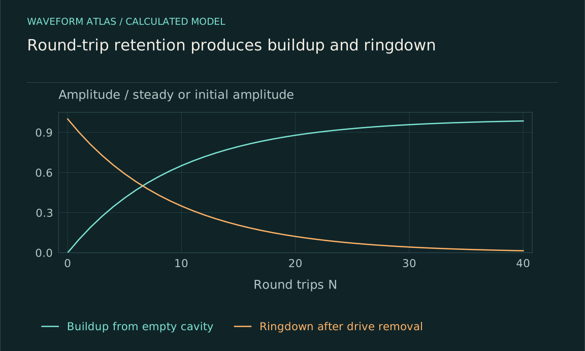
After N round trips from an initially empty cavity, the ideal field is proportional to [1−(r exp(iφ))ᴺ]/[1−r exp(iφ)]. At resonance, it approaches the steady value as rᴺ decreases. A high-retention cavity can produce a large steady field but takes many round trips to approach it. The same retention that creates strong buildup also creates memory of earlier input.

Turn the drive off and the stored field decreases by r each round trip, while stored energy decreases by r². This ringdown is a direct time-domain signature of the energy storage. A single-pass interference maximum does not necessarily show such a decay. Measuring the response after a drive interruption therefore provides information that a steady bright image or frequency scan alone cannot supply.

For r=0.9 at exact resonance, the steady geometric amplitude factor is ten. After ten round trips it is (1−0.9¹⁰)/0.1≈6.51, still well below its eventual value. Reaching 95 percent of the steady amplitude requires about 29 round trips because 0.9²⁹≈0.047. These numbers describe the amplitude sum for a fixed coupled input and should not be read as a tenfold total-power gain.

When the input stops, the stored amplitude falls to 0.9²⁹ of its initial value after the same 29 round trips, and the stored energy falls to its square. The different amplitude and energy decay rates are another reason to specify which ringdown is plotted. A graph labeled only decay time can obscure a factor of two even when the underlying cavity model is correct.

A mechanical oscillator gives another resonance model

Consider m ẍ+b ẋ+kx=F₀cosωt. The steady displacement amplitude is F₀/√[(k−mω²)²+(bω)²]. The response becomes large where the restoring and inertial terms nearly balance, with damping limiting the amplitude. Its phase relative to the force changes across the frequency range, determining how much average work the drive supplies.

Writing ω₀²=k/m and 2β=b/m, the displacement-amplitude peak occurs at √(ω₀²−2β²) when that expression defines a positive-frequency maximum. It is not exactly ω₀ at finite damping. Other observables, such as velocity amplitude or absorbed power, can peak differently. The phrase resonant frequency must therefore identify the response being measured, rather than treating every peak convention as identical.

With β/ω₀=0.1, the displacement peak is at about 0.9899ω₀, close to but measurably below the undamped frequency in a sufficiently precise experiment. With stronger damping the shift grows, and beyond the appropriate threshold no positive-frequency displacement maximum remains. A broad response can still be described by the oscillator model even when calling it a sharp resonance is unhelpful. The mathematical response function is more precise than a visual judgment about whether a curve looks peaked.

Energy storage distinguishes the sustained response

At steady state, the oscillator's average input power equals its average dissipated power. Near resonance, energy can circulate between kinetic and potential forms while the drive replaces losses. The large motion is not created by adding two externally prescribed waves at one point; it is the dynamical response of a system that stores energy and is continually driven.

A cavity has the analogous balance among incident coupling, leakage, internal loss and stored field energy. A lossless undamped model driven exactly on resonance can exhibit secular growth rather than a finite steady state, but that idealization does not imply every real resonator diverges. Finite drive duration, damping, detuning, nonlinearity and saturation determine what actually happens. The assumptions must accompany any claim of unlimited buildup.

Bandwidth and settling time are linked

A weakly damped resonance typically has a narrow response band and a long ringdown. In the standard oscillator convention, Q≈ω₀/(2β), the near-resonant half-power bandwidth is approximately 2β in angular frequency, and the amplitude envelope decays approximately as exp(−βt). These relationships apply in the stated regime and use half-power rather than half-amplitude width.

A single-pass interferometer's spectral fringe spacing instead depends primarily on path delay in its simplest model. That spacing is not automatically a resonator linewidth or a quality factor. Both systems can be frequency selective, but their transfer functions encode different physical memories. Comparing spectral width with time-domain decay helps distinguish a true stored-energy mode from interference between delayed copies.

Constructive interference is not automatically synchronization

A passive resonator can oscillate at the drive frequency after transients decay because the forced solution follows the drive. Synchronization usually concerns adjustment of an autonomous oscillator's rhythm through coupling or forcing. Such an oscillator has a sustained cycle without the external timing signal, supported by its own energy supply. A passive damped oscillator instead returns to rest when its drive is removed.

Likewise, two coherent inputs can reinforce because they were split from a common source, without mutually adjusting their frequencies. Their observed phase relation does not establish synchronization dynamics. The appropriate control is to examine uncoupled behavior and the response to detuning or coupling changes. This separates phase alignment imposed by preparation from a dynamical locking process.

Compare the mechanisms experimentally

For a suspected resonator, measure a calibrated input-output transfer function over frequency and record the decay after switching off or changing the drive. Look for a consistent model of linewidth, phase response and ringdown. For a single-pass interference experiment, scan relative phase and monitor complementary outputs or the spatial pattern at stable input power. The resulting signatures answer different questions.

A system containing both a cavity and an interferometer may require both tests. A dark output can result from cancellation between prompt reflection and a leaking stored field, while the internal energy remains large. Measuring only that output can hide the resonator's state. Include enough channels or time-resolved observables to separate internal buildup from external routing before assigning the enhancement or suppression to one mechanism.

Use the shared phase idea without erasing distinctions

Resonant buildup can be understood as repeated contributions arriving with a favorable phase. That connection makes interference a useful explanatory tool. The additional ingredients are feedback or repeated interaction, storage, loss and a dynamical response to changing drive. A bright region formed in one pass does not automatically possess those properties.

The practical conclusion is to name both the addition rule and the system dynamics. State which amplitudes reinforce, where energy is stored, how it enters and leaves, and which observable peaks. With those elements explicit, constructive interference and resonance fit into one consistent wave description while retaining the different measurements and engineering tradeoffs that make each concept useful.

Go to the original work.

These links identify the sources behind specific claims. Verification scope varies by source and is stated below.

1. 1 / University teachingMIT: Mach–Zehnder interferometers and beam splitters ↗

   MIT: Mach–Zehnder interferometers and beam splitters. https://ocw.mit.edu/courses/8-04-quantum-physics-i-spring-2016/resources/mach-zehnder-interferometers-and-beam-splitters/

   Beam splitters combine quantum path amplitudes.

   Verification scope: Official course record inspected; the matrices and worked examples here are independently specified.

2. 2 / University teachingOpenStax: Forced Oscillations ↗

   OpenStax: Forced Oscillations. https://openstax.org/books/university-physics-volume-1/pages/15-6-forced-oscillations

   A driven oscillator balances forcing, inertia, stiffness and damping.

   Verification scope: University textbook section inspected. This article derives exact peak and half-power conventions rather than adopting the section’s simplified peak and width wording.

3. 3 / University teachingFrequency response: Resonance, Bandwidth, Q factor ↗

   M. Chaniotakis and D. Cory (2006). Frequency response: Resonance, Bandwidth, Q factor. MIT OpenCourseWare 6.071J/22.071, Spring 2006.

   Quality factor, stored energy and half-power bandwidth for a specified circuit model.

   Verification scope: Official PDF first-page heading and course/author footer checked; the visible document title replaces its misleading embedded PDF metadata title.