Why reinforcement can fade with delay

Delay compares a field with its earlier self

A split-source interferometer can compare a field E(t) with a delayed copy E(t−τ). At zero delay, the two copies can share a highly stable relationship. At a longer delay, source frequency fluctuations or a broad spectrum can make their relative phase less predictable over the measurement. The phase-dependent enhancement then weakens in the averaged detector signal.

This is a statement about a correlation at a particular delay, not a claim that the delayed field has run out of energy. Each arm can retain the same average power while the cross term decreases. The MIT optical demonstration descriptions include path difference and coherence length as controls on fringe contrast. A quantitative interpretation additionally needs the source statistics, detector averaging and mode overlap used in the experiment.

Define normalized first-order coherence

For a stationary scalar field, define g¹(τ)=⟨E*(t)E(t+τ)⟩/⟨|E(t)|²⟩. Stationarity makes the correlation depend on delay rather than absolute start time. Its magnitude is at most one. With equal arm powers and perfect spatial and polarization matching, a controlled phase scan at delay τ has visibility |g¹(τ)|.

The maximum intensity at that delay is 2I₀[1+|g¹(τ)|], while the minimum is 2I₀[1−|g¹(τ)|]. Their sum is 4I₀ in this local two-contribution normalization. A fading maximum is accompanied by a rising minimum, not necessarily by falling arm powers. Measuring both extrema and the separate arms distinguishes loss of coherence from simple attenuation or a drifting source intensity.

The spectrum determines the stationary correlation

Under the usual stationary-field conditions, the correlation is the Fourier transform of the power spectral density. Using ordinary frequency ν, g¹(τ) is the normalized integral of S(ν)exp(i2πντ) over frequency. Different spectral components accumulate different phases as delay increases. Their phasor sum can shorten even though their individual spectral powers remain present.

This relationship is exact only for the specified correlation and spectrum conventions. It does not say that every finite pulse can be treated as a stationary random source, nor that an intensity-only spectrum supplies the complete phase of a deterministic pulse. A coherent chirped pulse can have a broad spectrum with controlled spectral phase. Distinguish stationary coherence measurements from pulse-shape reconstruction before using bandwidth as a universal synonym for randomness.

A Lorentzian example gives an exponential envelope

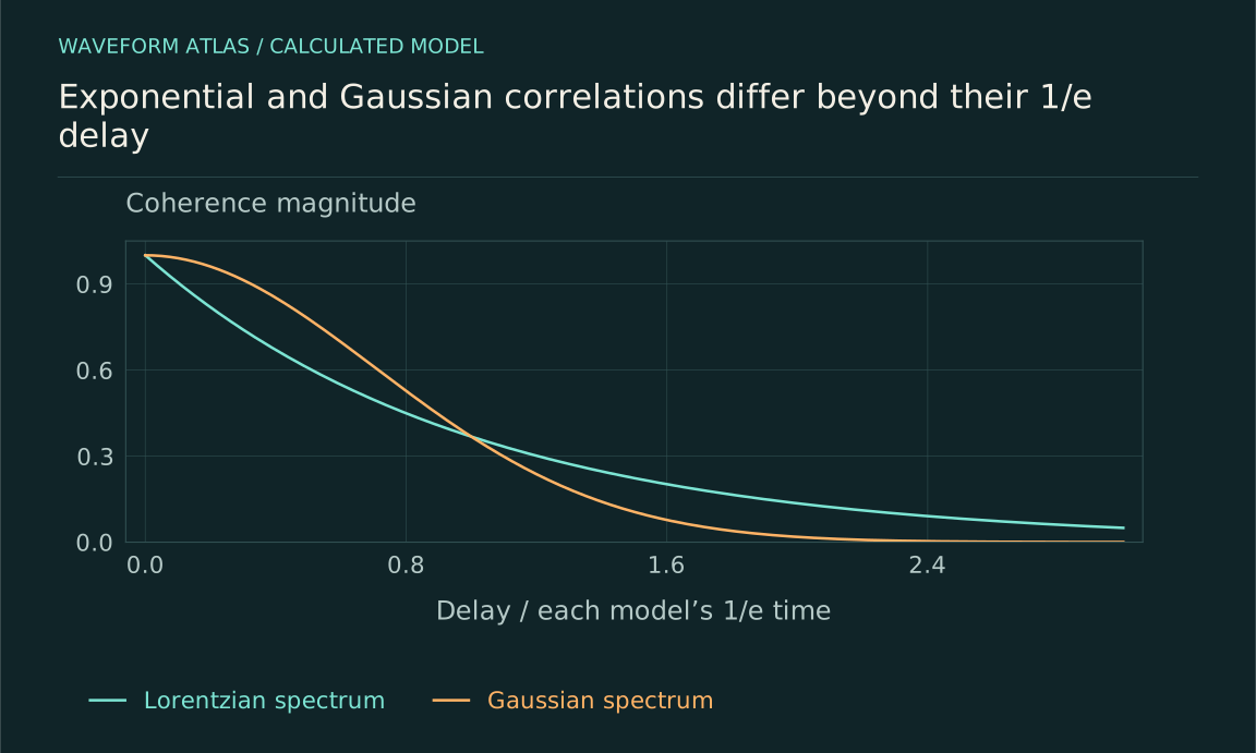
Take an ideal Lorentzian power spectrum centered at ν₀ with full width at half maximum Δν. Its normalized correlation is g¹(τ)=exp(i2πν₀τ)exp(−πΔν|τ|). Defining coherence time as the 1/e delay of the magnitude gives τc=1/(πΔν). A different definition, such as an integrated squared correlation, would produce a different numerical convention.

For Δν=1 megahertz, τc is about 0.318 microseconds. In vacuum, the corresponding path difference cτc is approximately 95.4 metres using c≈3×10⁸ metres per second. These are calculated values for an ideal spectral model. They do not claim that every one-megahertz source has this coherence length, because actual line shape, drift and measurement protocol can change the result.

At the Lorentzian 1/e delay, the ideal equal-arm maximum is 2I₀(1+1/e)≈2.736I₀ and the minimum is approximately 1.264I₀. Their visibility is 1/e even though the maximum still exceeds either arm's individual intensity substantially. This illustrates why simply observing a bright output is a poor quantitative measure of coherence: the noninterfering intensity background remains when the cross term is small.

A useful experimental normalization subtracts the independently measured sum of arm intensities from the combined signal and compares the remaining modulation with 2√(I₁I₂). That procedure isolates the cross term under the stated assumptions. It also makes uncertainty in background and arm-power measurements visible. Without those checks, an apparent long-delay plateau in the maximum can be mistaken for persistent coherence when it is mostly the unavoidable sum of individual powers.

A Gaussian spectrum gives a different decay

For a Gaussian spectrum with standard deviation σν, the normalized coherence magnitude is exp(−2π²σν²τ²). Its 1/e time is 1/(√2πσν). The spectral full width at half maximum is 2√(2ln2)σν. Combining those definitions gives a different numerical bandwidth-time product from the Lorentzian case, even when both widths are described casually as linewidth.

The distinction is measurable. At twice the respective 1/e time, a Gaussian envelope is exp(−4), while an exponential envelope is exp(−2). A sufficiently broad delay scan can distinguish them. Fitting a narrow portion of the data may not. Report the assumed line shape and uncertainty rather than converting a single fitted time into a linewidth without stating the model used for that conversion.

Coherence can revive instead of simply decay

Consider an ideal spectrum containing two equal infinitely narrow lines separated by δν. Its normalized correlation is a carrier phase times cos(πδντ). The visibility magnitude oscillates between zero and one. At some delays the two spectral contributions cancel in the correlation; at later delays they realign. A first zero is therefore not necessarily the end of all coherent reinforcement.

Finite linewidths would place an envelope around those revivals. A frequency comb or structured spectrum can produce more complicated correlation features. These examples show why a single coherence length can hide important spectral structure. Plot the full measured delay dependence when it is nonmonotonic, and distinguish a correlation zero caused by spectral phasor cancellation from irreversible disappearance of the underlying field.

Mode overlap can imitate a shorter coherence scale

Changing delay may also change alignment, beam size or polarization if the delay stage is imperfect. Those changes reduce the measured cross term independently of temporal coherence. A moving mirror can introduce beam walk; a dispersive element can alter spectral phase and polarization; unequal arm losses change the visibility baseline. The measured envelope is then a product or combination of several effects.

Monitor individual arm powers and overlap throughout the scan. Reverse the scan direction to check drift and hysteresis, and compare with a reference source or geometry when feasible. If a model attributes all contrast change to S(ν), it must justify why the other overlap factors remain controlled. A good spectral prediction is not enough if the apparatus changes the compared modes as delay varies.

Independent sources need a relative-frequency model

Two independent nominally equal-frequency sources can show a beat signal if their frequency difference lies within the detector bandwidth. Their relative phase evolves with the difference frequency and any additional noise. A long integration may average the beat term away even when each source is individually narrowband. A split-source delay experiment and an independent-source comparison therefore measure different relationships.

Phase locking the sources or recording a beat reference can restore a stable comparison in an appropriate frame. That is an active control or analysis resource, not proof that the original averaged signal contained a stationary bright fringe. State which reference is used and how its phase is tracked. Coherence is always defined for a pair of fields or alternatives and an observable comparison, not merely by assigning each source a label.

Measure the envelope without losing the carrier information

At each delay, scan a controlled phase through a full cycle or use quadrature detection to estimate the complex correlation. A single intensity reading versus delay mixes the rapidly varying carrier fringe with the slower visibility envelope. Detector resolution, stage calibration and phase jitter can blur those features differently. Extracting an envelope requires a method that separates them explicitly.

Compare the measured correlation with a separately measured spectrum using consistent normalization and frequency units. Account for finite spectrometer resolution, which can hide narrow features that matter at long delays. Conversely, a limited delay range restricts spectral resolution in an interferometric reconstruction. The two measurements provide complementary checks, and disagreement can reveal drift, nonstationarity or an incorrect assumption about the source's line shape.

For a finite scan, the largest measured delay sets how finely nearby spectral features can be separated in the reconstructed spectrum. The delay sampling interval sets another constraint on the spectral range represented without aliasing. These reciprocal limits follow from Fourier sampling and should be included when comparing an interferometric spectrum with a direct spectrometer. A smooth reconstruction can reflect a short observation window rather than proof that the physical spectrum has no narrow structure.

Interpret finite coherence operationally

Finite coherence means that a specified correlation weakens over a specified delay range and averaging procedure. It can limit how strongly delayed contributions reinforce without reducing their individual powers. The exact time or length depends on spectrum, reference, mode matching and definition. A broad spectrum need not imply an uncontrolled deterministic pulse, and a correlation zero need not forbid later revival.

The useful result states the measured g¹ or visibility envelope, the source model and the conversion to any quoted coherence length. That keeps constructive interference connected to the actual delay experiment. It also prevents a fading bright fringe from being mistaken for absorption, a new collapse mechanism, or a universal distance beyond which a wave ceases to exist.

Go to the original work.

These links identify the sources behind specific claims. Verification scope varies by source and is stated below.

1. 1 / University teachingMIT: Demonstrations in physical optics ↗

   Demonstrations identify amplitude, polarization, vibration, path difference and spectrum as controls on fringe contrast.

   Verification scope: Official course demonstration index and descriptions inspected.

2. 2 / University teachingMIT: Fraunhofer diffraction; Fourier transforms and theorems ↗

   Far-field diffraction relates aperture fields to Fourier transforms under stated approximations.

   Verification scope: Official lecture record and transcript excerpts inspected; aperture examples here are independently calculated.