A bright region belongs to a larger interference pattern

A point cannot describe the whole field

Two coherent waves do not generally reinforce everywhere. Their relative propagation phase changes with position, so one region can be bright while a nearby region is dark. A detector placed at a maximum samples one part of that pattern. Moving the detector can change its reading without changing either source's individual output. The spatial distribution is therefore part of the phenomenon, not an optional illustration.

This observation resolves many apparent energy puzzles, but it must be applied with a defined geometry. Some arrangements route power between discrete ports; others redistribute angular intensity; still others alter source loading. The statement that bright regions are balanced by dark regions is exact only within an appropriately complete, normalized propagation model. A local field formula alone does not specify every source and boundary contribution.

Derive a two-plane-wave pattern

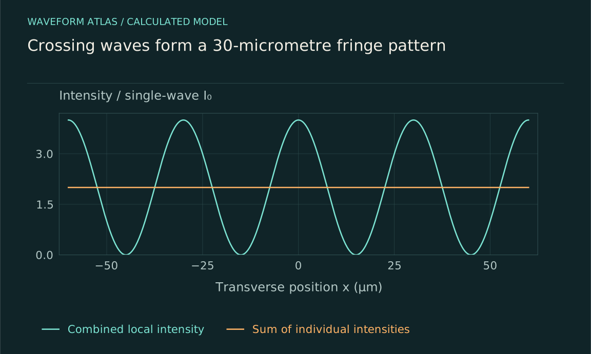
Consider two equal scalar plane-wave contributions crossing symmetrically at small angles ±θ to a common propagation axis. In a transverse plane, their phases differ by 2k x sinθ, where k=2π/λ. Under the scalar paraxial intensity approximation, the sum gives I(x)=2I₀[1+cos(2kx sinθ)]=4I₀cos²(kx sinθ). The fringe period is d=λ/(2sinθ).

For λ=600 nanometres and θ=0.01 radians, d is approximately 30 micrometres. Each contribution alone supplies I₀ in this local normalization, while maxima reach 4I₀ and minima reach zero. These values describe ideal infinite waves and a chosen observation plane. A finite experimental beam adds an envelope, and exact electromagnetic flux uses the Poynting vector rather than treating every geometry as a scalar intensity.

Average over complete fringe periods

Integrating the ideal pattern over an integer number of periods gives an average of 2I₀, the sum of the individual contributions in the same approximation. The cosine cross term integrates to zero. A detector covering only a bright fraction can read an average above 2I₀, while one centered on a dark fraction can read below it. Detector area therefore changes the measured quantity.

For a centered interval of width L, the average cross term is proportional to sin(qL/2)/(qL/2), where q=2k sinθ. This sinc factor describes how finite-area integration suppresses the modulation. It is not an intrinsic loss of coherence. Resolving the same region with smaller pixels can recover the visible fringes even when a large-area detector reports almost no phase-dependent signal.

For a detector width equal to half a fringe period and centered on a bright maximum, qL/2=π/2, so the averaged cosine contribution is 2/π≈0.637. The mean signal is then 2I₀(1+2/π)≈3.273I₀. Center the same detector on a minimum and the mean becomes 2I₀(1−2/π)≈0.727I₀. The detector size and source powers are unchanged; only its location relative to the pattern differs.

These values are useful for checking a scanned detector against a resolved camera image. Integrating the camera pixels over the detector's actual aperture should reproduce its signal after calibration and resolution effects are included. A disagreement points to collection geometry, detector response or an inadequate field model before it points to any failure of energy conservation. This comparison connects a local pattern directly to a measurable finite-area power reading.

Finite beams add envelopes and boundaries

Real beams have finite widths, and the overlap region may cover only part of each beam. Outside that region, one contribution can exist without the other. A complete image therefore contains the interference pattern inside the overlap and individual-beam intensity elsewhere. Cropping the image to its brightest central region discards precisely the information needed for a global comparison.

The envelope can also vary across a fringe, so the simple integer-period cancellation becomes approximate. Use the measured or modeled field profiles in the integral rather than assuming a uniform background. If the beams are clipped by apertures, the apertures introduce diffraction and possible loss. The power removed by clipping belongs in the budget and should not be attributed to destructive interference in the remaining image.

Fourier propagation makes normalization explicit

In a suitable far-field or focal-plane approximation, the output field is proportional to a Fourier transform of the aperture field. The constants depend on wavelength, distance or focal length, and the coordinate convention. When input and output modes are normalized consistently, propagation through an ideal lossless optical system preserves the appropriate field norm. Phase changes reshape the output without necessarily changing the input intensity.

A discrete unitary Fourier transform offers a transparent teaching model. For N input amplitudes aⱼ, define bₖ=(1/√N)Σaⱼexp(−i2πjk/N). Then Σ|bₖ|²=Σ|aⱼ|² exactly. Setting all input phases equal can concentrate power in one output bin; changing phases redistributes it. The model shows the conservation relationship without pretending that a finite camera captures every physical direction of a real apparatus.

A four-mode example tracks every output

Take input amplitudes (1,1,1,1) in a four-mode unitary transform. The output amplitudes are (2,0,0,0), so all four units of power reach the first mode. Change the input to (1,1,−1,−1), and the power moves into other output combinations while the sum remains four. The details follow from the transform, not from a rule that bright fields must create energy.

This discrete example is a mode-accounting model, not a literal four-pixel photograph of two slits. Its strength is that every channel is included and the normalization is explicit. A physical implementation may have additional modes and losses, which must be added before comparing with measured efficiency. The same discipline applies to a continuous spatial pattern: define what constitutes the complete set of outgoing channels.

Directional intensity and flux are different

For an electromagnetic field, energy flow is described by the Poynting vector. For sound, intensity involves pressure times particle velocity. A local squared field amplitude is often proportional to intensity for a single traveling mode, but standing waves and crossing fields can require more careful interpretation. A bright electric-field region does not by itself specify the direction or amount of net energy crossing every surface.

Choose a surface and integrate the normal component of the appropriate energy-flux vector when making a total-power claim. In paraxial optics, camera irradiance can be an excellent practical proxy on a perpendicular plane, but the approximation should be stated. This is especially important when comparing fields at large angles or near reactive sources, where a simple scalar intensity picture can hide relevant components.

Sources and boundaries can change the balance

If two radiators are driven with fixed motion or fixed current, their mutual fields can alter the work required from the drives. Changing relative phase may therefore change total radiated power as well as its angular distribution. A source model that prescribes fields without tracking the drive cannot simultaneously guarantee unchanged input work. The missing energy term is then in the source interaction, not outside conservation.

Boundaries can also store or dissipate energy. A nearby reflector changes the radiation pattern and source impedance; an absorbing wall converts some wave energy to other forms. A spatial interference map should be interpreted within those boundaries. The simple lossless Fourier model is a useful baseline, but it is not a substitute for the complete physical system when experimental conditions include feedback, absorption or time-dependent storage.

Design a spatial measurement that can discriminate

Record each source separately and both together using the same calibrated detector settings. Scan relative phase and collect an area large enough to include the relevant pattern and envelope. Compare the measured combined image with the field-model prediction, including detector resolution and background. A spatially integrated quantity should state its exact collection boundary and any power known to lie outside it.

Repeat after shifting the detector aperture or changing beam angle. Fringe spacing should follow the geometry, while the integrated cross term should respond to the collection window. Monitor source powers during the scan to distinguish redistribution from changes in emitted power. These controls turn a bright image into a quantitative test of interference and make clear which part of the energy account the camera actually observes.

Interpret enhancement as a distribution change

A bright region is evidence that contributions add constructively there under the measured conditions. Its significance depends on what happens elsewhere and what the sources supply. In a normalized lossless mode model, enhanced power in one region or channel is accompanied by redistribution across the rest. In a driven-source problem, changed source work can also matter. Both descriptions obey the same conservation requirement.

The useful conclusion is therefore spatially explicit: this phase arrangement concentrates a defined fraction of input power into this measured region. Such a statement can guide focusing, beam shaping and sensing without turning a local maximum into a claim of net amplification. The full pattern provides the context that a single bright pixel cannot supply.

Go to the original work.

These links identify the sources behind specific claims. Verification scope varies by source and is stated below.

1. 1 / University teachingOpenStax: Interference of Waves ↗

   Linear superposition and phase-dependent addition of mechanical waves.

   Verification scope: University textbook section inspected.

2. 2 / University teachingMIT: Fraunhofer diffraction; Fourier transforms and theorems ↗

   Far-field diffraction relates aperture fields to Fourier transforms under stated approximations.

   Verification scope: Official lecture record and transcript excerpts inspected; aperture examples here are independently calculated.