The basic resonance model

State the equation and its units

Use m ẍ+b ẋ+kx=F₀cosωt. Here x is displacement, m is mass, b is a viscous damping coefficient, k is spring stiffness, F₀ is force amplitude and ω is drive angular frequency. The model assumes a restoring force proportional to displacement and a damping force proportional to velocity. It describes one effective coordinate with parameters that remain constant over the experiment.

Writing ω₀²=k/m, 2β=b/m and f=F₀/m gives ẍ+2βẋ+ω₀²x=fcosωt. This normalized form is convenient, but f has units of acceleration and β has units of inverse time. Keep angular frequency in radians per second distinct from ordinary frequency in hertz. The conversion ω=2πν matters when interpreting linewidths, periods and phase accumulation.

Solve using a complex response

Represent the force as the real part of F₀exp(iωt) and seek x as the real part of Xexp(iωt). Substitution gives X=F₀/[k−mω²+i bω]. The complex susceptibility χ(ω)=X/F₀ contains both amplitude and phase. Its magnitude is 1/√[(k−mω²)²+(bω)²], and its argument determines the displacement lag.

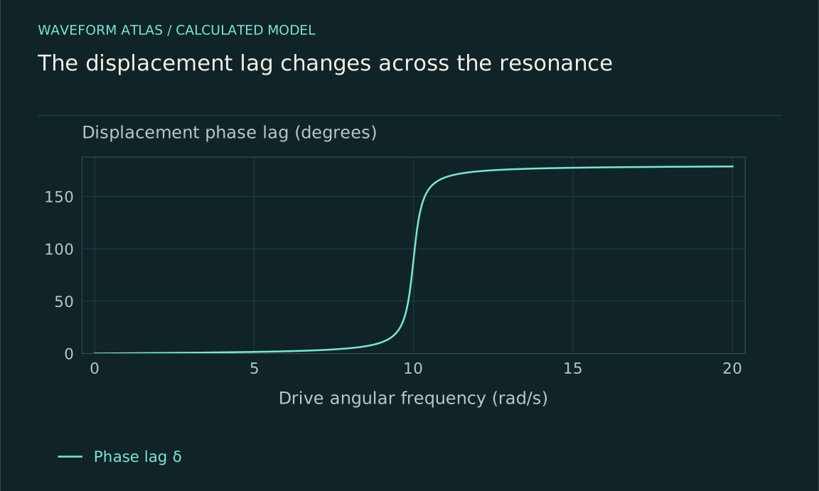
Thus x(t)=Acos(ωt−δ), with A=F₀|χ| and δ=atan2(bω,k−mω²). The two-argument arctangent keeps the correct quadrant across resonance. A plain arctangent of a ratio can accidentally lose the approach toward π at high frequency. The complex formula avoids that ambiguity and makes it straightforward to compare phase-sensitive measurements with the model.

Interpret three frequency regimes

When ω is much smaller than ω₀, inertia is weak and A≈F₀/k. Displacement follows the force nearly in phase, like a slowly loaded spring. Near ω₀, the stiffness and inertial terms nearly cancel, leaving damping to set the response scale. At ω=ω₀, A=F₀/(bω₀) and the displacement lag is π/2.

When ω is much larger than ω₀, inertia dominates and A≈F₀/(mω²). Displacement is nearly opposite in phase to the force. These limits provide useful checks on a fitted transfer function. A curve that does not approach the appropriate low- and high-frequency behavior may include actuator response, another mode, a different measured variable or a failure of the assumed one-coordinate model.

Locate the displacement maximum exactly

The squared denominator in normalized units is D(ω)=(ω₀²−ω²)²+4β²ω². Differentiating gives D′(ω)=4ω(ω²−ω₀²+2β²). A nonzero-frequency amplitude maximum therefore occurs at ωr=√(ω₀²−2β²), provided ω₀²>2β². For sufficiently strong damping, the displacement response decreases from its zero-frequency value without a separate positive-frequency maximum.

This exact result explains why calling ω₀ the displacement resonance is an approximation at finite damping. In the weak-damping limit the difference is small, so the shorthand can be useful if its regime is understood. In precision work, specify whether frequency means the undamped natural frequency, damped free-oscillation frequency, displacement peak or another response peak. They are related but not generally identical.

Velocity and power peak differently

The velocity amplitude is ωA. For constant force amplitude and constant viscous damping, its maximum occurs at ω₀. The average dissipated power is P̄=bω²A²/2, so it also peaks at ω₀, reaching F₀²/(2b). This differs from the displacement-amplitude peak because multiplying by ω changes the frequency dependence.

The measured sensor output may be proportional to displacement, velocity, acceleration or a mixture. A voltage peak is therefore not enough to identify which mathematical resonance was observed. Calibrate the transduction and compare the appropriate transfer function. This distinction becomes especially important when a mechanical sensor is read electrically and its electronics introduce additional frequency dependence or phase shifts.

Verify the energy balance

Define mechanical energy E=m ẋ²/2+kx²/2. Differentiating and using the equation of motion gives dE/dt=F(t)ẋ−b ẋ². The first term is work supplied by the drive, and the second is dissipated power. In periodic steady state, the average stored-energy change is zero, so average input work equals average dissipation.

During buildup or ringdown, dE/dt is not zero. A temporary mismatch between input and dissipated power changes stored energy. This equation is the correct place to track that difference rather than assuming every cycle is already in steady balance. It also shows explicitly that the large resonant response is powered by the drive; the oscillator does not create energy because its natural and drive frequencies are close.

Add the transient solution

The full motion is the steady forced solution plus a homogeneous solution fixed by initial conditions. In the underdamped case, the latter is exp(−βt)[Ccos(ωdt)+Dsin(ωdt)], with ωd=√(ω₀²−β²). The constants ensure the initial displacement and velocity are satisfied. At critical or overdamping, the homogeneous form changes and should not be represented by an oscillation with an imaginary frequency on a real plot.

A frequency sweep that does not wait for these transients can show apparent asymmetry or lag unrelated to a nonlinear steady-state response. After a drive switch, beating between the transient and forced components can occur. Record enough time to distinguish the settling process from the final sinusoid. The steady susceptibility is a frequency-domain result whose experimental use requires an appropriate observation window.

The transient frequency ωd and its envelope rate β can be estimated from a free-decay record after the drive is removed. Combining them gives ω₀²=ωd²+β² in the underdamped model. Those independently estimated parameters predict the driven susceptibility, including its slightly shifted displacement maximum. Agreement between the two measurements is a useful test that the damping and stiffness remained unchanged.

A changing amplitude during ringdown can alter frequency in a nonlinear oscillator, invalidating a fit to one fixed ωd. Likewise, a sum of two nearby modes can produce beats that resemble a varying envelope. Inspect the residuals and instantaneous timing of zero crossings before interpreting every nonexponential decay as an unusual damping law. The single-mode model should earn its use through these consistency checks.

Work a numerical example

Let m=1 kilogram, k=100 newtons per metre, b=0.4 newton-seconds per metre and F₀=0.01 newtons. Then ω₀=10 radians per second and β=0.2 per second. At zero frequency, the displacement is 0.1 millimetres. At ω₀ it is 2.5 millimetres, with a quarter-cycle lag. The average dissipated power there is 0.000125 watts.

The displacement peak is at √99.92≈9.996 radians per second, while the free damped frequency is √99.96≈9.998 radians per second. Their small difference is intentional in this weakly damped example. A plot with limited resolution may make all three frequencies look identical, but the definitions remain distinct. The calculated values should be checked against the actual linear range of any proposed mechanical implementation.

At the drive frequency ω₀, the velocity amplitude in this example is 0.025 metres per second. Its squared cycle average is half the square of that value, and multiplying by b=0.4 gives the stated dissipated power. The force and velocity are in phase there, so averaging their product gives the same value, F₀ω₀A/2. This independent calculation checks both the phase convention and the factor of one half from sinusoidal averaging.

If a measurement instead reports rms force and rms velocity, their product at this phase equals average power directly. Mixing peak amplitudes with rms amplitudes introduces another factor-of-two error. State the amplitude convention whenever numerical power is inferred from sinusoidal signals, particularly when comparing an oscilloscope trace with a meter that reports rms values.

Examine the zero-damping limit carefully

If b approaches zero away from resonance, the ideal steady amplitude approaches F₀/|k−mω²|. At exact resonance, the steady-state expression is singular because no finite periodic solution balances continuous resonant work without loss. Starting from suitable zero conditions, the undamped resonant solution contains (F₀/2mω₀)t sinω₀t, whose amplitude grows with time.

This limit does not predict instantaneous infinite displacement. It predicts secular growth under exact tuning and an indefinitely valid linear model. Any finite experiment has a duration, and real systems generally have losses or nonlinear effects that eventually matter. The correct interpretation is to solve the initial-value problem in the relevant regime, not to insert zero damping into a steady-state denominator and treat infinity as an observed physical event.

Test where the model stops working

Measure amplitude and phase at several drive strengths. In the linear regime, the complex response X/F₀ should be independent of F₀. Harmonics, amplitude-dependent frequency shifts, hysteresis or saturation indicate additional dynamics or instrument limitations. Check the actuator and detector as well as the oscillator, because either can generate apparent nonlinearity.

A successful fit should describe multiple observables, such as displacement response and ringdown, with consistent parameters. When it fails, identify the missing ingredient: another mode, nonviscous damping, nonlinear stiffness, feedback or changing boundary conditions. The simple driven oscillator remains a useful baseline because every assumption is visible and each deviation suggests a concrete measurement that can refine the model.

Go to the original work.

These links identify the sources behind specific claims. Verification scope varies by source and is stated below.

1. 1 / University teachingOpenStax: Forced Oscillations ↗

   OpenStax: Forced Oscillations. https://openstax.org/books/university-physics-volume-1/pages/15-6-forced-oscillations

   A driven oscillator balances forcing, inertia, stiffness and damping.

   Verification scope: University textbook section inspected. This article derives exact peak and half-power conventions rather than adopting the section’s simplified peak and width wording.