What ringdown says about resonator losses

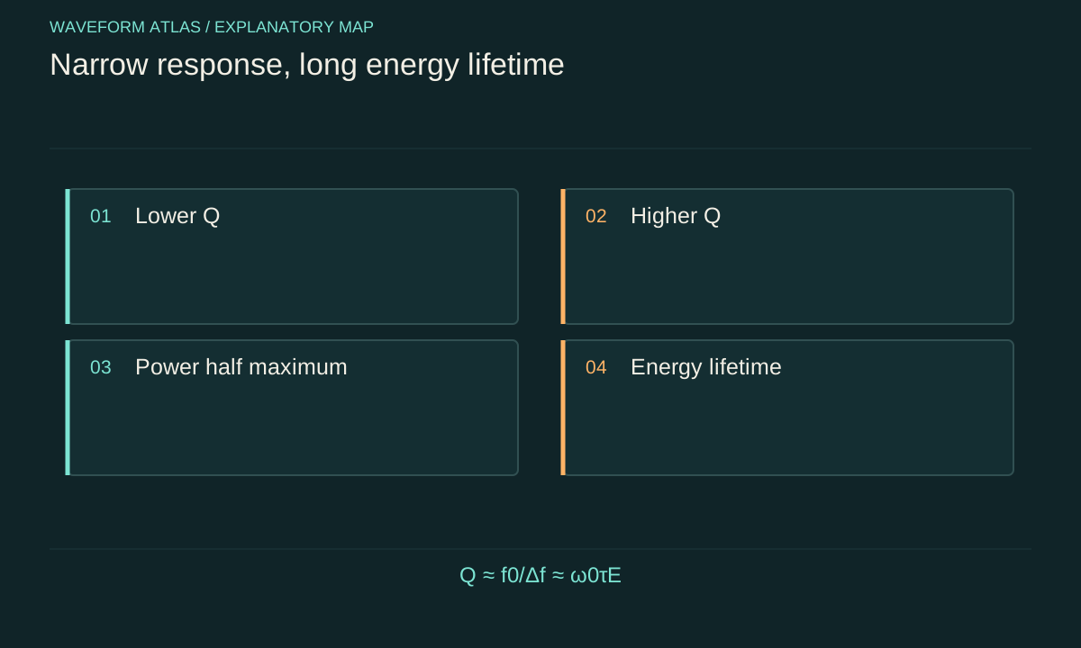
What the ratio measures

A resonator can store substantial energy while losing only a small fraction each cycle. Quality factor expresses that comparison in dimensionless form. In the weak-loss limit, Q ≈ 2πU/ΔUcycle, where U is stored energy and ΔUcycle is energy lost over one oscillation. Large Q means the energy persists through many cycles relative to the oscillation period.

The word quality is historical and does not mean that larger Q is always preferable. A high-Q resonator can provide narrow frequency selectivity and strong field buildup, but it also responds slowly and retains unwanted excitation after a drive ends. A broadband receiver, rapidly switched actuator, or vibration suppressor may need a lower Q. The appropriate design depends on the task. Q is most useful when it names a specified mode, frequency, and operating condition rather than serving as a universal score for a device.

Derive the ringdown connection

Suppose stored energy follows U(t) = U0 exp(−κt). Its lifetime is τE = 1/κ. Over one period T0 = 2π/ω0, the fractional loss is 1−exp(−κT0). If κT0 is small, this is approximately κT0, so the cycle definition gives Q ≈ ω0/κ = ω0τE.

The approximation matters. At strong damping, the energy changes appreciably during one cycle, and the idea of a sharply defined oscillation can become poor. The exact finite-cycle energy ratio contains the exponential rather than its first-order expansion. Different generalized definitions of Q need not agree outside the narrow-resonance regime. When quoting Q from a ringdown, give the fitted energy lifetime and resonance frequency as the primary measurements. Readers can then see the assumptions behind the derived dimensionless number and compare it with other conventions.

Amplitude lifetime produces a different formula

For the viscously damped oscillator, displacement has an envelope exp(−γt), while cycle-averaged energy decays approximately as exp(−2γt). Thus τA = 1/γ and τE = τA/2. The weak-damping relation becomes Q ≈ ω0τA/2, not ω0τA. A direct intensity measurement and an amplitude-sensitive measurement can therefore produce slopes differing by two without any physical disagreement.

Consider a 2-kilohertz resonator whose measured displacement envelope has a 0.10-second lifetime. Its energy lifetime is approximately 0.05 second, giving Q ≈ 2π × 2,000 × 0.05 ≈ 628. Using the amplitude lifetime as though it were the energy lifetime would report about 1,257. This simple error can survive sophisticated fitting. A measurement description should explicitly identify whether the fitted quantity is displacement, field amplitude, intensity, power, or stored energy.

Linewidth is another view of the same response

An isolated linear resonance with exponential free decay has a Lorentzian-like frequency response near its peak. For the usual power-response full width at half maximum Δf, Q ≈ f0/Δf. The energy-decay rate κ corresponds to an angular-frequency linewidth, so Δf = κ/(2π) in the narrow-resonance model.

For the preceding example with Q ≈ 628 at 2 kilohertz, the expected power linewidth is about 3.18 hertz. A frequency sweep must resolve that scale without changing the resonator's state or averaging over significant drift. A linewidth of an amplitude curve is not numerically identical to a power half-maximum linewidth. The horizontal axis units also matter: hertz and radians per second differ by 2π. Giving the measured curve and width convention is more useful than quoting Q alone, especially when different instruments are being compared.

Loaded and internal quality factors differ

A resonator loses energy internally and through deliberate coupling to external ports. If their independent decay rates add, κloaded = κinternal+κexternal. Since Qj = ω0/κj under the same convention, 1/Qloaded = 1/Qinternal+1/Qexternal. The loaded value describes the assembled experiment, including the measurement or output connection.

For an illustrative internal Q of 10,000 and external Q of 10,000, the loaded Q is 5,000. Improving the internal material loss alone cannot make the loaded Q exceed the external-coupling limit. Conversely, weakening the probe can increase the measured loaded Q while reducing signal extraction. This is not a contradiction; the probe is part of the energy budget. Multiple ports add further inverse-Q terms only when the independent-channel model applies. Coherent feedback and frequency-dependent environments may require a more complete response model.

A high value does not locate the loss

A measured Q gives a total loss scale for the selected mode. It does not identify whether energy escapes as radiation, enters a support, heats a material, or converts into another mode. Two devices can have the same Q with very different microscopic mechanisms and temperature sensitivities. Their performance may diverge under a change of frequency, amplitude, or mounting conditions.

To identify the cause, vary one coupling or material parameter at a time and measure additional channels. Changing an optical output coupler tests leakage. Changing support geometry tests mechanical radiation. Temperature dependence can help constrain internal relaxation mechanisms, though it is rarely unique evidence by itself. Spatial mode shapes reveal where strain or field energy is concentrated. Q is the beginning of loss diagnosis, not its conclusion. A useful report distinguishes a directly measured total decay rate from an inferred internal-loss contribution.

Frequency noise can broaden a measured line

A resonator whose instantaneous frequency wanders can produce a broad averaged response even if its energy decays slowly. A frequency sweep samples both energy relaxation and the distribution of resonance frequencies during acquisition. Depending on the measurement, phase fluctuations can therefore reduce apparent spectral sharpness without an equivalent increase in energy loss.

Compare time-domain ringdown with frequency-domain linewidth and repeat both over different acquisition times. If a faster sweep gives a narrower line or repeated traces shift in frequency, drift is a plausible contributor. Phase-sensitive ringdown measurements also require care because phase wandering can reduce an averaged coherent amplitude. Measuring energy separately helps distinguish this from actual stored-energy decay. Calling every linewidth an energy lifetime assumes a stationary single-mode model. The distinction is especially important when Q is used to infer a material loss coefficient or compare coherence with relaxation.

Amplitude dependence marks a model boundary

A linear resonator has an approximately amplitude-independent frequency and damping rate over its operating range. At larger excitation, stiffness can change, heating can alter material response, and damping can become nonlinear. A single Q then may not describe the entire ringdown. The early, high-energy part can decay differently from the late, weak-motion part.

Measure Q or the underlying decay rate at several initial amplitudes and report the range over which it is stable. Check that the detector remains linear, since saturation can create a false amplitude dependence. A driven frequency sweep may also show hysteresis or a shifted resonance when nonlinear dynamics become important. In that case, reporting the response curve and preparation history is more informative than forcing one linewidth formula onto it. A scalar Q remains useful locally, but its conditions must accompany it.

Uncertainty follows both frequency and lifetime

If Q = 2πf0τE and the frequency and lifetime estimates are independent, the relative standard uncertainty is approximately the square root of the sum of their squared relative uncertainties. A frequency known to 0.01 percent and a lifetime known to 2 percent produce a Q uncertainty dominated by the lifetime. More digits in f0 will barely improve the result.

Systematic effects often exceed the statistical uncertainty of an exponential fit. Residual drive, baseline error, detector filtering, and an incorrect fit interval can bias τE. Correlated errors require a covariance term rather than independent quadrature addition. A practical uncertainty budget should separate repeatability from calibration and model assumptions. Report the raw lifetime, observable, and fitting procedure alongside Q so another researcher can reassess the result if the decay model or coupling interpretation changes.

Use Q to make a design decision

The stored-energy time sets a settling timescale. In the exponential model, reducing energy to one percent requires t = τE ln(100) ≈ 4.61τE. A device with a 10-millisecond energy lifetime therefore needs about 46 milliseconds to reach that residual level after a clean shutdown, unless an active extraction or additional damping path changes the dynamics.

This calculation turns a quality factor into a concrete operational consequence. High Q can improve selectivity while slowing switching; lower Q can broaden bandwidth while reducing buildup. The energy destination still matters when a damping path is added. An active cancellation of one observed field is not automatically removal of all stored energy. Specify the mode, threshold, and measurement channel when discussing settling. Q then becomes a transparent bridge between stored energy, spectral response, and the practical time needed for a resonator to become quiet.

The number of visible oscillations also depends on dynamic range. Even a fixed Q can yield a longer-looking trace when the initial amplitude is larger or the detector noise is lower. Counting cycles until the trace disappears is therefore not a calibrated Q measurement unless the visibility threshold and initial amplitude are controlled. Fitting a physical decay model uses more of the information.

Go to the original work.

These links identify the sources behind specific claims. Verification scope varies by source and is stated below.

1. 1 / University teachingDamped Oscillations — University Physics Volume 1 ↗

   OpenStax. University Physics Volume 1, Section 15.5: Damped Oscillations.

   Linear viscous damping and damping regimes

   Verification scope: Official textbook section and equation record inspected

2. 2 / University teachingFundamentals of Photonics: Quantum Electronics — lecture notes ↗

   Franz X. Kärtner. Fundamentals of Photonics: Quantum Electronics — lecture notes. 2006.

   Population dynamics, absorption/gain, Rabi oscillations and coupled modes

   Verification scope: Official author-written course materials and topic mapping inspected

3. 3 / University teachingOscillations: Key Equations — University Physics Volume 1 ↗

   Oscillations: Key Equations — University Physics Volume 1.

   Oscillator equations and amplitude/frequency conventions

   Verification scope: Official equation page inspected

4. 4 / Primary researchCavity ring-down spectrometer for high-fidelity molecular absorption measurements ↗

   H. Lin; Z. D. Reed; V. T. Sironneau; J. T. Hodges. Journal of Quantitative Spectroscopy and Radiative Transfer 161, 11–20 (2015).

   DOI: 10.1016/j.jqsrt.2015.03.026

   Exponential cavity decay fitting, baseline offsets and a loss budget separating mirror loss, etaloning, scattering and absorption.

   Verification scope: NIST-hosted full text: title page and relevant decay-fit/loss-budget passages inspected; not every section reread.

5. 5 / Primary researchCoupled-cavity ring-down spectroscopy technique ↗

   J. B. Courtois; J. T. Hodges. Optics Letters 37(16), 3354–3356 (2012).

   DOI: 10.1364/OL.37.003354

   Controlled optical feedback changes a coupled cavity decay; reported ring-down time increases from 210 to 280 microseconds.

   Verification scope: NIST abstract and primary PDF bibliographic page inspected

6. 6 / University teachingWave Propagation — Triantaphyllos Akylas, lecture notes ↗

   Triantaphyllos Akylas. Wave Propagation — Triantaphyllos Akylas, lecture notes. 2017.

   Transient wave propagation, elastic modes, interfaces and water waves

   Verification scope: Official chapter contents and author-written course records inspected

7. 7 / University teachingElectromagnetics and Applications, Chapter 9: Electromagnetic Waves ↗

   David H. Staelin. Electromagnetics and Applications, Chapter 9: Electromagnetic Waves. 2009.

   Planar boundaries, complex media, waveguides and cavity resonators; §9.4 defines Q through energy loss and exponential decay.

   Verification scope: Current official PDF download verified; relevant chapter passages inspected, not an entire textbook reread.

8. 8 / University teachingSignals and Systems — Alan V. Oppenheim, lecture notes ↗

   Alan V. Oppenheim. Signals and Systems — Alan V. Oppenheim, lecture notes. 2011.

   Convolution, linear systems, filtering and feedback

   Verification scope: Official course notes and topic records inspected

9. 9 / University teachingQuantum Optical Communication — Jeffrey H. Shapiro, readings and lecture slides ↗

   Jeffrey H. Shapiro. Quantum Optical Communication — Jeffrey H. Shapiro, readings and lecture slides. 2016.

   Author-written quantum attenuator, amplifier, detection and parametric interaction framework

   Verification scope: Official course materials and topic mapping inspected