A shorter pulse can require a broader spectrum

The envelope is not the carrier cycle

An optical pulse can be represented by a rapidly oscillating carrier multiplied by a more slowly varying complex envelope. The envelope describes when most of the energy arrives, while the carrier frequency describes the rapid field oscillation. Shortening the envelope does not automatically increase the carrier frequency. A pulse can become temporally narrower while remaining centred on essentially the same optical frequency.

The distinction depends on the bandwidth and the approximation used. For very short pulses containing only a few cycles, separating carrier and envelope requires additional care. Even in that regime, duration and central frequency remain different descriptors. Report the field or intensity quantity used to define duration, its width convention and the spectrum. A single number called pulse length cannot characterize every physically relevant feature of the waveform.

Fourier components need both magnitude and phase

Write the spectral envelope as Ã(Ω)=|Ã(Ω)|exp[iφ(Ω)], where Ω is frequency relative to a chosen carrier. The spectral magnitude identifies how much of each frequency is present. The phase determines how those components combine in time. Different spectral phases can produce different temporal envelopes while leaving the spectral intensity unchanged. A spectrometer alone therefore cannot establish that a pulse is as short as its bandwidth permits.

A common phase adds no change to the envelope intensity. A phase term linear in Ω shifts the pulse in time. Quadratic and higher terms alter the relative arrival timing and can broaden or reshape the pulse. These distinctions are useful when diagnosing a compressor: a delay is not failed compression, while residual phase curvature can prevent a pulse from reaching the duration expected from its spectrum.

Define the transform-limited reference

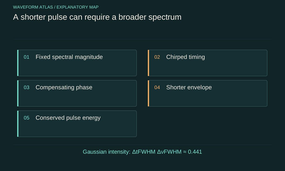
For a given spectral magnitude, a transform-limited pulse has aligned spectral phase after removing irrelevant constant and linear terms. The exact duration depends on the spectral shape and on how width is defined. For an intensity-Gaussian pulse, the full-width-at-half-maximum time–frequency product is approximately 0.441 when ordinary frequency, rather than angular frequency, is used. Other shapes and conventions produce different numerical factors.

This relation is a Fourier property, not a universal statement that every pulse has that product. Chirp and other phase structure increase the duration for the same Gaussian spectral magnitude. A spectrum with sidebands or several separated lobes can produce temporal satellites, making a single width insufficient. Compare the complete measured or reconstructed envelope with the appropriate transform-limited reference instead of inserting every spectrum into a Gaussian formula.

Work through a bandwidth estimate

An ideal Gaussian intensity pulse with 100-femtosecond full width at half maximum requires approximately 4.41 terahertz of frequency bandwidth at the transform limit. A 50-femtosecond pulse of the same shape requires approximately 8.82 terahertz. These are calculated examples, not measured specifications of a device. They use the same width convention for both temporal intensity and spectral intensity.

The example explains the careful wording shorter can require broader. A chirped 200-femtosecond pulse might already contain bandwidth sufficient for 100 femtoseconds. Removing its chirp can reach that shorter duration without creating new frequencies. But going substantially below the transform limit set by its existing spectral magnitude requires a change in bandwidth or waveform definition. A passive phase-only compressor cannot manufacture arbitrary missing spectral content.

Chirp correlates frequency with time

A chirped pulse has a time-dependent instantaneous frequency within an appropriate complex-field description. Different spectral components can be delayed relative to one another, stretching the envelope. A compressor applies a compensating frequency-dependent delay so that those components overlap more closely. The sign and magnitude of compensation must match the incoming phase rather than follow a universal rule that any dispersive element shortens a pulse.

In an illustrative Gaussian model, a dimensionless chirp parameter C gives an intensity duration enlarged by √(1+C²) relative to its unchirped reference under the corresponding parameterization. At C=√3, the duration doubles. Here define the spectral amplitude as Ã(Ω)∝exp[−T₀²Ω²/2]exp[iCT₀²Ω²/2]. Its inverse Fourier transform has intensity ∝exp[−t²/(T₀²(1+C²))], so its FWHM is 2√ln2 T₀√(1+C²). The physical point is that the longer duration can reside in phase organization rather than in a narrower spectral magnitude.

A compressor is a physical optical system

Gratings, prisms and dispersive materials can impose frequency-dependent phase. Their geometry and material response determine the available compensation, transmission and bandwidth. A system optimized for one spectrum may leave higher-order phase errors in another. Spatial dispersion, angular dispersion and coupling between position and frequency can also affect the pulse at the target, so a one-dimensional temporal model may be incomplete.

Measure the pulse where it will be used, after the relevant optics. A short pulse before a window can broaden after passing through it. A compressor output measured in one spatial region may differ from another if the beam has spatial–spectral structure. Report the collection aperture and target plane along with temporal characterization. These practical details connect a mathematical phase correction to the field that actually reaches the experiment.

Amplification and recompression are separate stages

The University of Rochester identifies Strickland and Mourou's 1985 work on compression of amplified chirped optical pulses as the origin of chirped-pulse amplification. The sequence stretches a pulse, amplifies it at lower peak intensity, and recompresses it. The historical record supports that mechanism and publication attribution. It does not mean that a passive compressor itself supplies the energy added by the amplifier.

Keep those stages separate in the energy ledger. Stretching at nearly fixed energy lowers peak power; amplification adds energy from a pumped medium; recompression concentrates the surviving energy into a shorter interval. Real stages introduce losses and imperfect phase control. Comparing only the final peak power with the initial peak power would mix energy gain with temporal concentration and conceal which part of the apparatus caused each change.

Calculate peak power with a shape factor

For a Gaussian intensity pulse P(t)=P_peak exp[−4 ln2 t²/τ²], where τ is the intensity full width at half maximum, integration gives energy U=P_peak τ√π/(2√ln2). Thus P_peak is approximately 0.9394 U/τ. The familiar energy divided by duration is a useful scale, but the exact peak depends on pulse shape and width convention. Satellites and pedestals can further reduce the fraction of energy in the main peak.

For an illustrative one-microjoule, 100-femtosecond Gaussian pulse, this expression gives about 9.394 megawatts of peak power. If an ideal compressor halves the duration at fixed energy and shape, the peak doubles. This is not free energy: the time integral remains one microjoule. Actual transmission loss reduces the final energy and can offset some of the peak-power increase.

Measure phase as well as duration

A direct electronic detector may be too slow to resolve an ultrashort optical pulse. Nonlinear or interferometric characterization methods infer temporal structure through a known measurement process. Such an inference has assumptions about the gate, response, spatial overlap and retrieval procedure. An autocorrelation width alone does not uniquely determine every possible pulse shape, even though it can provide a useful duration estimate under a stated model.

Use a characterization method appropriate to the claim and verify its calibration. Compare spectrum, pulse energy and reconstructed temporal profile. Check for secondary pulses or a broad pedestal rather than reporting only the narrowest central feature. If phase retrieval is used, test consistency between the reconstructed field and the measured data. A visually narrow trace can otherwise overstate how much energy was successfully compressed into the useful pulse.

Distinguish compression from filtering and postselection

A spectral or temporal filter can select a portion of a pulse and produce a narrower displayed feature while discarding energy. That differs from coherent phase compensation applied to the full retained waveform. Likewise, a measurement that accepts only certain arrival times changes the selected ensemble without necessarily shortening every emitted pulse. Report the acceptance probability or energy fraction so the selection remains visible.

A phase-sensitive reversal or propagation test can help distinguish these mechanisms. If a known inverse phase restores the initial stretched field, the result supports coherent phase control within the tested bandwidth. Failure of reversal may arise from loss, nonlinear distortion or inaccurate compensation, so it does not uniquely identify fundamental decoherence. The full spectral and energy record is needed to decide which explanation fits the observation.

A complete report gives input and output energy, temporal intensity, spectral intensity and the phase information needed for the interpretation. It identifies the target plane, pulse shape convention, compression factor and useful main-pulse energy fraction. It also distinguishes measured data from a calculated transform-limited reference. Those quantities let another reader evaluate whether the device achieved phase compensation, bandwidth generation, filtering or some combination.

Pulse compression is therefore a controlled reorganization of a wave in time. It can preserve coherence and increase peak power without changing total energy in an ideal passive stage. Its limitations follow from bandwidth, phase control, propagation and losses. Keeping those variables separate makes a shorter pulse an understandable physical result, rather than a misleading suggestion that squeezing a temporal plot has extinguished or collapsed the wave.

Go to the original work.

These links identify the sources behind specific claims. Verification scope varies by source and is stated below.

1. 1 / Official researchUniversity of Rochester, Chirped-Pulse Amplification: 1985 ↗

   Institutional history identifies Strickland and Mourou’s 1985 paper; primary sequence is cited separately.

   Verification scope: Institutional text and cited-paper metadata inspected. The schematic’s full content was not assessed; no absence claim is made about the image.

2. 2 / Primary experimentStrickland and Mourou, Compression of amplified chirped optical pulses ↗

   Donna Strickland; Gerard Mourou. Optics Communications 56(3), 219–221 (1985).

   DOI: 10.1016/0030-4018(85)90120-8

   Original stretch–amplify–recompress sequence; the corrected 1985 publication.

   Verification scope: Publisher abstract/metadata verified; introductory sequence read from indexed text of the University of Toronto-hosted paper. Full-paper performance/uncertainty audit not performed.

3. 3 / University teachingKärtner, MIT 6.977 Ultrafast Optics, Chapter 2: Maxwell–Bloch Equations ↗

   F. X. Kärtner, MIT 6.977 Ultrafast Optics, Chapter 2, §2.8, Table 2.2 (Spring 2005).

   Linear dispersive propagation and §2.8, Table 2.2: Gaussian intensity FWHM time–bandwidth product 0.441. The article derives its chirp parameterization and peak-power factor.

   Verification scope: Pulse-propagation discussion and §2.8/Table 2.2 inspected, not the full textbook.