What changes when confinement varies with time?

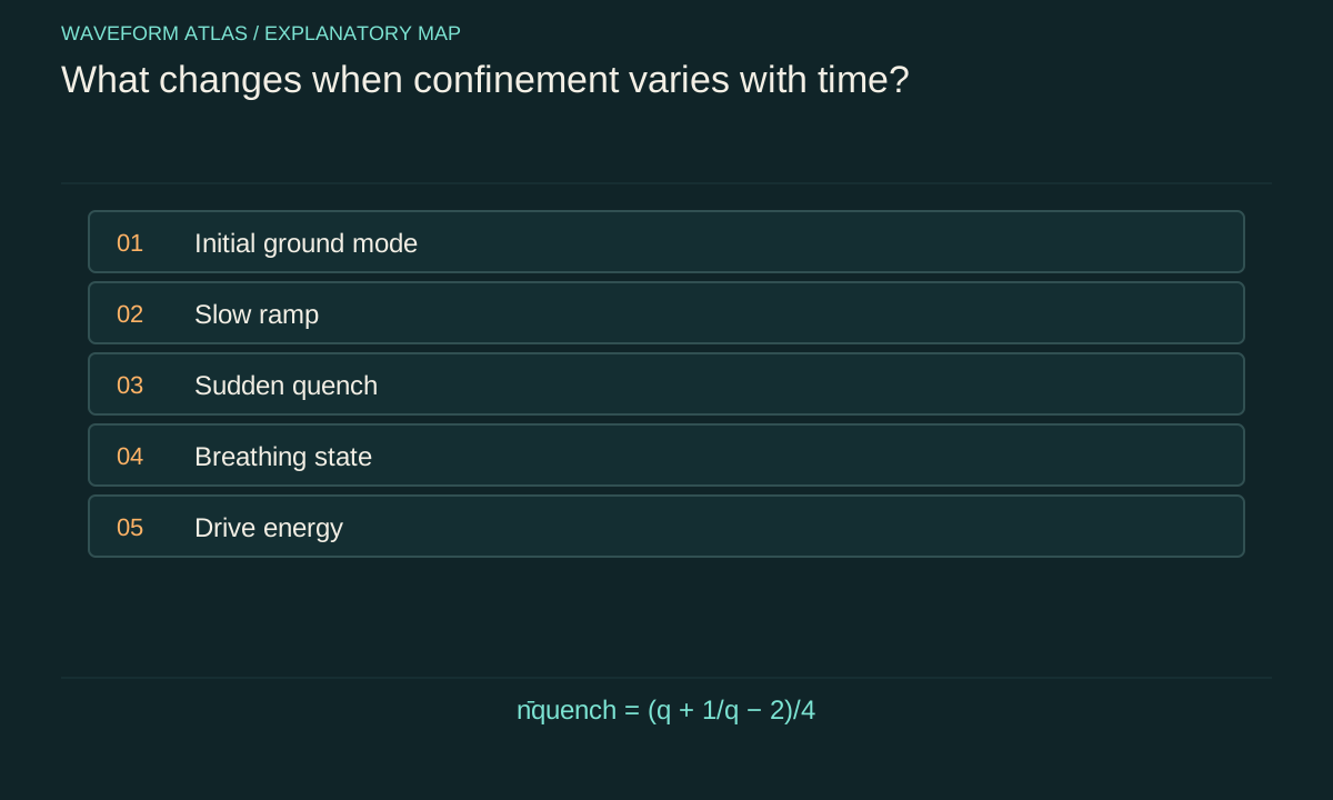
Geometry becomes a time-dependent control

A static cavity or trap defines a set of modes. When its boundary or restoring potential changes, those modes and their frequencies become functions of time. The state must evolve under the changing equations; it cannot be obtained merely by replacing the old width with the new width in a static picture. The control history determines how much of each final mode is occupied.

Represent the control by a measured function such as L(t) for a cavity length or ω(t) for a harmonic trap frequency. Include ramp duration, smoothness and any oscillations. Two controls with identical endpoints can produce different states because their intermediate histories differ. A reproducible experiment therefore needs more than a before-and-after photograph of the geometry. It needs the timing and calibration of the motion or effective boundary change.

Slow means slow relative to the system

Adiabatic following is an approximation in which a state initially occupying an isolated instantaneous eigenmode remains close to the corresponding evolving mode. The relevant condition involves the rate of Hamiltonian change, its coupling between modes and their energy gaps. A ramp that is slow for one pair of levels can be fast near a small gap. There is no universal duration that makes every confinement change adiabatic.

The state accumulates phase during this following, including relative phases if several modes were initially populated. Preserving mode populations therefore does not mean nothing happened. A phase-sensitive experiment can reveal the accumulated evolution even when final density resembles the initial shape after rescaling. When testing adiabaticity, examine both unwanted excitations and the observables relevant to the intended use, rather than relying only on a narrow final histogram.

A harmonic trap gives a solvable baseline

Consider H=p²/(2m)+mω²x²/2. Its ground-state position variance is ℏ/(2mω), and its momentum variance is ℏmω/2. If frequency doubles adiabatically, position variance halves and momentum variance doubles. The state remains the ground state of the instantaneous Hamiltonian in the ideal limit, while its energy rises from ℏω₀/2 to ℏω₀. The controller supplies that increase.

This narrowing is different from squeezing relative to a fixed oscillator Hamiltonian. The reference ground-state width itself changed. After returning frequency adiabatically to its initial value, the original widths can be recovered, together with an accumulated phase. State which Hamiltonian defines the reference when describing the final state as squeezed, excited or ground. Without that reference, identical-looking ellipses can receive inconsistent labels.

A sudden frequency change leaves a mismatch

In an ideal sudden change, the state does not have time to change during the switch, but the Hamiltonian changes. An initial ground state at frequency ω₀ is generally not the ground state at the new frequency ω₁. Its position and momentum variances are initially the old ones, so it becomes a coherent superposition of final energy eigenstates. Subsequent evolution can make the density breathe.

For q=ω₁/ω₀, the mean final excitation number in this ideal quench is (q+1/q−2)/4. If q=2, it is one eighth. The state remains pure under the closed-system unitary model despite occupying more than one final energy level. This calculated counterexample shows why added excitation cannot be treated as automatic evidence of decoherence or collapse. The excitation has a predictable phase structure.

Compare the work for two histories

For the sudden doubling example, the energy immediately after the switch is ℏω₀(1+q²)/4=1.25ℏω₀. Subtracting the initial 0.5ℏω₀ gives work input 0.75ℏω₀. The adiabatic doubling instead ends at energy ℏω₀, requiring work 0.5ℏω₀. Both protocols reach the same final trap frequency, but the sudden one leaves additional excitation.

These are ideal calculations for a single isolated harmonic mode, not experimental energy measurements. A real ramp takes finite time and can include damping, technical noise and coupling to other modes. Measuring the final energy distribution and ramp waveform allows comparison with a more realistic prediction. The endpoint geometry alone cannot identify how much work was done or whether the resulting state is close to the intended mode.

Parametric driving can amplify selected motion

A periodic modulation of a restoring parameter can exchange energy resonantly with a mode. The response depends on modulation frequency, phase and amplitude relative to the oscillator dynamics. Such driving can produce phase-sensitive amplification and squeezing in suitable regimes. It is not equivalent to applying a static force, nor does every modulation simply damp the wave. The control signal acts as an explicit energy source.

A useful analysis starts with a stable small-modulation regime and checks where the approximations fail. Large drive can excite additional modes, shift frequencies or create nonlinear response. Record the drive spectrum and look for output at frequencies beyond the original signal. A detector restricted to one narrow band can interpret frequency conversion as disappearance, even when energy has moved into other accessible channels.

An electrical boundary can emulate motion

Wilson and colleagues reported the dynamical Casimir effect in a superconducting circuit whose effective electrical boundary was rapidly modulated. The verified primary abstract describes generated microwave radiation and two-mode squeezing. The boundary change was implemented through circuit control, not by physically translating a metal mirror at the same effective speed. This distinction belongs in any visual or analogy used to explain the experiment.

The modulation supplies the energy of the emitted radiation. The result is evidence for a specified driven quantum-field process, not a claim of energy from an unchanged vacuum. It also demonstrates that altering confinement can create excitations rather than eliminate them. Our account is limited to the primary abstract and does not reconstruct the full experimental calibration or assert that every moving-wall system produces detectable radiation.

Physical walls introduce additional degrees of freedom

A mechanical boundary has mass, elasticity and internal modes. Moving it can excite vibrations, heat or electromagnetic noise that couple to the confined field. An effective fixed-boundary approximation may be adequate in one regime and fail in another. Include the controller and boundary dynamics when their backreaction affects the observable. The field and wall can exchange both energy and momentum.

The actual motion may differ from the commanded waveform because of inertia, resonances or feedback delay. Measure the boundary trajectory independently where possible. A discrepancy between predicted and observed field response may originate in that control transfer function. Treating the command voltage as the exact wall position can otherwise create an apparent unexplained excitation or loss that disappears once the mechanical response is included.

Reversal must reverse the relevant dynamics

Returning a boundary to its initial position does not necessarily undo the state evolution. The state may have accumulated mode-dependent phases or exchanged energy with other degrees of freedom. An inverse operation must compensate the actual transformation, including timing, rather than merely repeat the geometry in reverse order. In a closed system that inverse can exist mathematically even if it is difficult to implement experimentally.

Use calibrated control sequences and compare with numerical evolution under the measured Hamiltonian. A successful recovery of phase-sensitive observables supports reversible control within the tested range. An unsuccessful recovery is informative only after known control errors and environmental coupling are assessed. It does not uniquely identify a fundamental reduction process, because ordinary unitary evolution followed by an inaccurate inverse can produce the same failure.

Design a rate-dependent test

Prepare a known initial mode and vary ramp duration while keeping the endpoint confinement fixed. Measure final mode populations, moments and a phase-sensitive observable. Add an unchanged control and a recovery sequence. Monitor temperature, transmission and the actual control waveform so that heating or loss is not silently assigned to geometry. Compare the measured dependence with the predicted slow and fast limits.

The most useful graph places the control rate on an axis alongside a declared response such as excitation number or recovery fidelity. Label calculated curves and measured points separately. A minimum in excitation may reflect an optimized control sequence rather than monotonic improvement with slower motion, so test the relevant range. The conclusion should identify the dynamical regime and remaining noise, preserving the distinction between coherent excitation and irreversible environmental effects.

The sudden-quench formula gives zero added excitation when q=1, as required for an unchanged oscillator. It is symmetric under q→1/q for the dimensionless excitation number, although the physical energies are referenced to different final frequencies. Near q=1+ε, the excitation begins at approximately ε²/4, so very small deterministic frequency changes create a second-order excitation in this ideal model. These limits provide quick checks on algebra and numerical implementations.

They do not remove the need to model a finite ramp. A calculation should reproduce both the no-change limit and the appropriate sudden or adiabatic limits before being used to interpret intermediate rates. Such checks are more informative than a smooth animation because they connect the displayed response to conservation, normalization and known dynamical behaviour.

Go to the original work.

These links identify the sources behind specific claims. Verification scope varies by source and is stated below.

1. 1 / University teachingMIT Quantum Physics I: lecture notes ↗

   Course materials cover normalization, observables, wells, scattering and angular momentum.

   Verification scope: Official course index inspected; linked lecture topics verified.

2. 2 / Primary experimentWilson et al. (2011), Observation of the dynamical Casimir effect in a superconducting circuit ↗

   A modulated superconducting circuit produced radiation with two-mode squeezing; energy is supplied by modulation.

   Verification scope: Primary-paper abstract in PubMed inspected; DOI 10.1038/nature10561 verified.

3. 3 / University teachingAdams, MIT Quantum Physics I: Optional Problems on the Harmonic Oscillator ↗

   Coherent states, uncertainty, sudden oscillator-frequency changes and time-dependent squeezed-state quadratures.

   Verification scope: Official six-page problem sheet text inspected, including frequency-change and quadrature questions; original worked examples in our articles.