Who supplies or receives the work of compression?

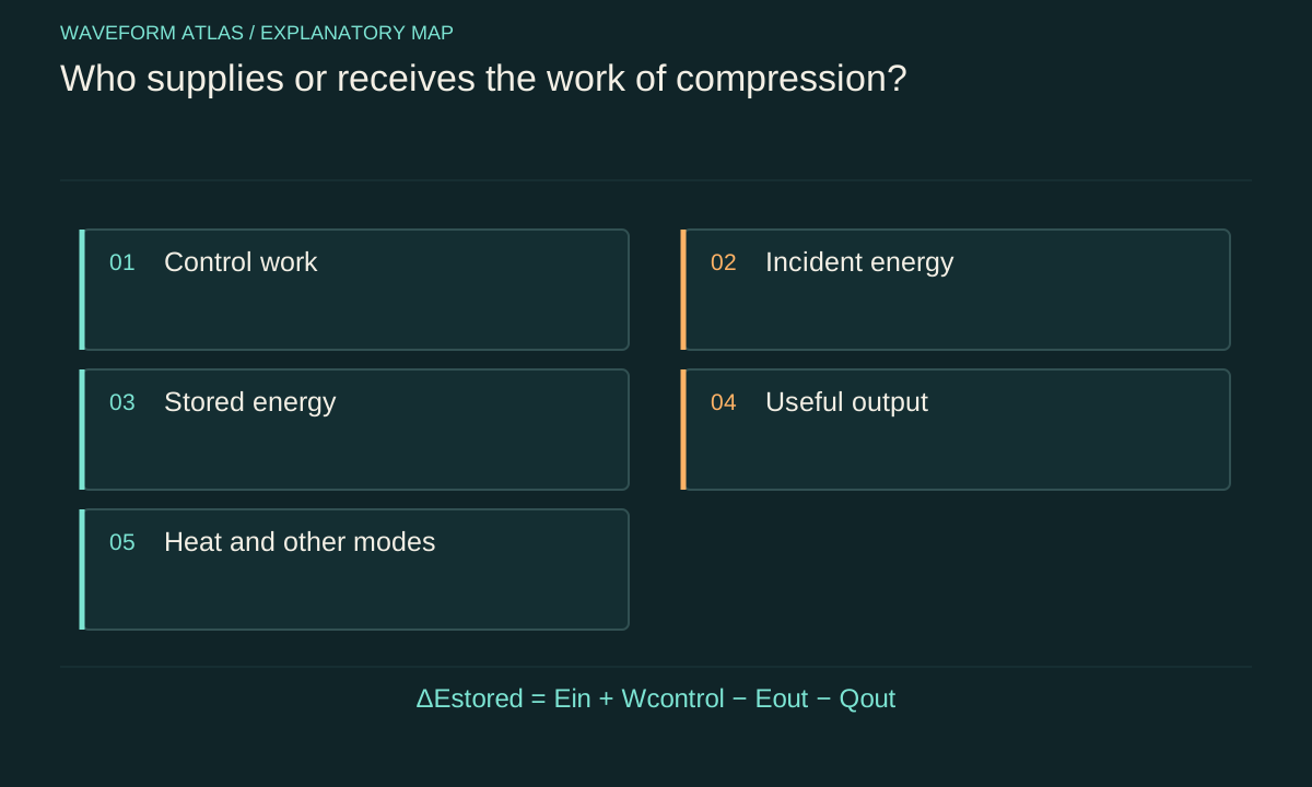
Choose a system boundary

Energy accounting begins by defining which components belong to the system. A field alone, a field plus cavity walls, and the entire apparatus including power supplies have different energy flows across their boundaries. None is automatically the correct choice; the useful choice is the one that makes the proposed claim testable. State the boundary and include every channel crossing it over the observation interval.

For a driven cavity, those channels may include mechanical work from an actuator, electromagnetic input and output, absorption in the walls and changes in stored field energy. For a compressed gas, include heat exchange and internal energy. A detector in one output channel measures only part of that ledger. A reduction in its reading cannot identify the total energy change without the remaining terms.

A changing Hamiltonian supplies a general relation

For a closed quantum system evolving unitarily under H(t), the change of mean energy is d⟨H⟩/dt=⟨∂H/∂t⟩. The commutator contribution from the state’s evolution cancels when evaluating the energy expectation. Explicit parameter changes therefore describe work supplied by the control within this ideal model. If the Hamiltonian is time independent, the mean energy remains constant even while the probability density changes shape.

An open system adds energy exchange through coupling to unobserved degrees of freedom. Separating work and heat can depend on the model and on how the system boundary is chosen, especially for strong coupling. For an introductory ledger, state the weak-coupling or effective assumptions used and keep the measured total balance clear. A convenient label should not conceal a physically real exchange with the environment.

For an explicitly time-dependent observable A, the product rule adds ⟨∂A/∂t⟩ to the Lecture 8 commutator result: d⟨A⟩/dt=⟨∂A/∂t⟩+(i/ℏ)⟨[H,A]⟩. Setting A=H makes the commutator vanish. This extension is derived here; the cited lecture itself treats observables without explicit time dependence.

A stiffness change depends on the state

For a classical oscillator with energy p²/(2m)+kx²/2, an abrupt stiffness change δk at fixed instantaneous x and p changes energy by δk x²/2. The same control step therefore does different work at different phases of the motion. Applied at a displacement node it can do little instantaneous work; applied near maximum displacement it can do much more. Geometry or stiffness change alone does not determine the energy transfer.

In a quantum state, the corresponding expectation involves ⟨x²⟩. A state with zero mean position can still have nonzero ⟨x²⟩ and receive work from the stiffness change. This connects energy accounting to fluctuations rather than only to mean displacement. Record the state preparation and timing when comparing control sequences, since equal endpoint parameters do not guarantee equal work.

Tightening an ideal well raises mode energy

For a nonrelativistic particle in an ideal one-dimensional infinite well, E_n∝L^(−2). Halving the width while preserving the mode index raises its energy by a factor of four. The work required in the adiabatic eigenstate comparison is three times the initial energy. This positive input is consistent with the outward generalized force associated with the energy’s dependence on width.

The result is a specific model, not a universal sign rule for compression. A rapid protocol can add further excitation, and a finite barrier can introduce loss or coupling to other modes. If the experiment reports only the surviving population after compression, include the energy and probability of rejected or escaped events. Otherwise the apparent average energy of survivors can obscure a substantial exchange with unmeasured channels.

Closing an attractive gap can release work

For ideal Casimir plates, interaction energy per area is negative and becomes more negative as the gap decreases. A controller restraining the attractive motion can in principle receive work during a quasistatic closure. This differs from tightening the infinite well because the energy landscape is different. The word compression does not fix the direction of energy transfer; the relevant Hamiltonian or interaction energy does.

Reopening the plates along the reverse ideal path requires returning that energy. A complete cycle includes the actuator, electrical conditions and losses. If material properties are changed between stages, include the energy needed for those changes. A favourable segment of a cycle cannot establish net energy production when the preparation and reset stages have been omitted from the account.

Pulse compression changes power concentration

A passive ideal pulse compressor can shorten a pulse while preserving its energy. The peak power then rises because the same energy arrives in a shorter interval. For a fixed pulse shape, reducing duration by a factor of two doubles peak power. This is temporal concentration, not energy amplification. The integral of power over time is the quantity to compare when testing energy conservation.

Chirped-pulse amplification includes an actual amplifier between stretching and recompression stages. That amplifier obtains energy from its pump. Keep its gain separate from the compressor’s phase correction and losses. A final high peak power can result from both added pulse energy and reduced duration. Reporting only the peak does not reveal their relative contributions or the energy consumed by the overall system.

Stored energy can delay the output

During a transient, incident energy can accumulate in a cavity or material excitation before leaving later. A short measurement window may therefore show less outgoing energy than incoming energy without implying absorption or disappearance. Integrate long enough to include ringdown, or independently estimate the stored-energy change at the end of the interval. The appropriate duration depends on the system’s decay times.

The reverse situation is also possible: an output pulse can exceed the contemporaneous input because it releases previously stored energy. Include the preparation stage that filled the storage. A comparison limited to the brightest moment can hide that history. Time-resolved energy accounting distinguishes gain supplied by a drive, release from storage and redistribution of an input pulse.

Momentum belongs beside energy

A reflected wave changes momentum and can exert force on a boundary. A boundary moving under that force exchanges mechanical energy at a rate related to force times velocity. The apparatus support can receive momentum even when it does little work because its displacement is small. Thus energy conservation alone does not settle a claim about recoil, thrust or force.

Include the actuator, supports and outgoing radiation or material flow in the momentum balance when those quantities matter. A wave redirected into an unmeasured angle can carry momentum away even if its energy is nearly unchanged. Compression or mode conversion does not remove that requirement. A complete physical account should not imply unbalanced propulsion merely because a selected field channel became weaker or narrower.

Loss is an exchange, not a missing category

Absorption transfers organized field energy into material degrees of freedom, often followed by heat flow. Scattering redirects energy into other modes. Detector inefficiency leaves some outcomes unrecorded. These mechanisms can all reduce a measured signal, but their ledgers differ. Calling every reduction loss may be convenient operationally, yet the physical explanation requires naming the destination or bounding the unmeasured channels.

Measure complementary outputs and backgrounds where feasible, and propagate their uncertainties. If the remaining deficit is comparable with combined uncertainty, do not assign it a precise physical mechanism. A thermal measurement can support absorption, while expanded angular collection can reveal scattering. The useful next measurement is the one that closes the specific unresolved part of the budget.

A hypothetical ledger clarifies the test

Suppose a driven process receives one joule in an incoming pulse and 0.2 joule of control work. Afterward, 0.8 joule leaves in the desired output, 0.1 joule in other outgoing modes, 0.2 joule becomes heat and 0.1 joule remains stored. The total output and storage is 1.2 joules, matching the input. These are hypothetical numbers illustrating categories, not experimental data or a proposed device specification.

If a report measured only the desired output, it might describe a twenty-percent reduction from the incident pulse while overlooking the added drive work and other channels. If it later released the stored energy, that output would need to be assigned to the same complete history. A ledger with explicit time boundaries prevents such selective comparisons and reveals which measurements remain missing.

For a claimed cyclic process, compare complete initial and final states of the working system, controller and relevant reservoirs. If a battery discharges, a gas cools or a strained support relaxes, the cycle consumed a resource even if the visible wave returned to its original shape. Repeating the sequence requires restoring that resource. Include reset work and losses in the total efficiency.

The final conclusion should identify the measured energy transfers and their uncertainty, not merely the direction in which a drawing became narrower. Compression can store work, release interaction energy, concentrate power or dissipate motion depending on the mechanism. Following the complete balance makes those possibilities compatible with ordinary conservation laws and supplies a direct test for any additional claim that proposes a different energy accounting.

Keep the sign convention beside the ledger. Work delivered by the controller is positive input here; a controller receiving work contributes a negative value to that same term.

Go to the original work.

These links identify the sources behind specific claims. Verification scope varies by source and is stated below.

1. 1 / ReviewDecca, Aksyuk and López, Casimir Force in Micro and Nano Electro Mechanical Systems ↗

   R. Decca, V. Aksyuk and D. López, Casimir Force in Micro and Nano Electro Mechanical Systems, in Casimir Physics, Lecture Notes in Physics 834, 287–309 (Springer, 2011), doi:10.1007/978-3-642-20288-9_9.

   DOI: 10.1007/978-3-642-20288-9_9

   Ideal parallel-conductor pressure and importance of real-material, surface and geometry corrections.

   Verification scope: Springer chapter metadata and abstract verified; NIST-hosted chapter introduction and ideal pressure equation used. Entire chapter not audited.

2. 2 / Official researchUniversity of Rochester, Chirped-Pulse Amplification: 1985 ↗

   Institutional history identifies Strickland and Mourou’s 1985 paper; primary sequence is cited separately.

   Verification scope: Institutional text and cited-paper metadata inspected. The schematic’s full content was not assessed; no absence claim is made about the image.

3. 3 / Primary experimentStrickland and Mourou, Compression of amplified chirped optical pulses ↗

   Donna Strickland; Gerard Mourou. Optics Communications 56(3), 219–221 (1985).

   DOI: 10.1016/0030-4018(85)90120-8

   Original stretch–amplify–recompress sequence; the corrected 1985 publication.

   Verification scope: Publisher abstract/metadata verified; introductory sequence read from indexed text of the University of Toronto-hosted paper. Full-paper performance/uncertainty audit not performed.

4. 4 / University teachingZwiebach, MIT 8.04 Lecture 8: Time dependence of expectation values ↗

   Barton Zwiebach (2016). 8.04 Lecture Note 8. https://ocw.mit.edu/courses/8-04-quantum-physics-i-spring-2016/72de1b688f3f40e1c42b26b3da29585a_MIT8_04S16_LecNotes8.pdf

   Section 3, Eq. (3.37), gives the commutator contribution for an observable with no explicit time dependence. The article explicitly derives any added time-derivative term.

   Verification scope: Section 3 read; the notes explicitly restrict their derivation to time-independent observables.