Compressing the carrier rather than the wave

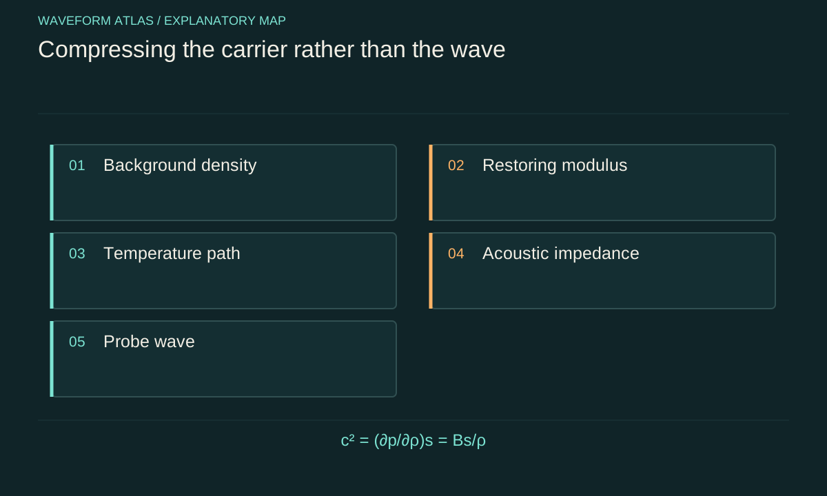
Separate the background from the disturbance

A small sound wave is a perturbation around a material's background pressure, density and temperature. Compressing the entire sample changes that background. The wave then propagates through a different state of matter. Its own alternating compressions and rarefactions are smaller perturbations superimposed on that state. Confusing these two levels makes it easy to treat a slow piston movement as though it were simply increasing the amplitude of every acoustic oscillation.

Record the background variables before and after the intervention, and define the wave amplitude relative to the local equilibrium. A pressure sensor may see a large offset from the piston plus a much smaller oscillating component. Separating those signals requires a calibrated measurement with enough dynamic range. Removing the offset in software can be appropriate, but it should not conceal the physical work and heating associated with changing the background.

Sound speed comes from a derivative

For a simple fluid under the appropriate small-signal conditions, c²=(∂p/∂ρ)_s, where the derivative is taken at constant entropy for an adiabatic acoustic perturbation. Equivalently c²=B_s/ρ, with B_s the adiabatic bulk modulus. The derivative describes how strongly pressure responds to a small density disturbance. Density supplies inertia, but the restoring response can change at the same time.

This formula does not say that compressing every material slows its waves. If stiffness rises sufficiently, the speed can increase even while density rises. The derivative must correspond to the relevant frequency and thermodynamic regime. Heat exchange or internal relaxation during the oscillation can modify the effective response. Use the material law appropriate to the perturbation, not merely the path used to prepare the compressed background.

Isothermal preparation can leave ideal-gas speed unchanged

For an ideal gas of fixed composition, the usual adiabatic small-signal sound speed is c=√(γRT/M), where γ is the heat-capacity ratio and M the molar mass. Compressing the background isothermally raises pressure and density in the same proportion. If temperature, composition and γ remain fixed, this ideal sound speed remains unchanged. The acoustic perturbation can still be approximately adiabatic even though the slow background preparation exchanged heat.

This distinction between preparation path and perturbation derivative is important. Saying the gas was compressed isothermally does not automatically mean every acoustic wave should be analysed with an isothermal modulus. The wave frequency and heat-transfer timescale determine its effective response. State both processes separately. A real gas or a frequency range with significant relaxation can depart from the elementary ideal-gas prediction.

Adiabatic preparation gives a different result

For reversible adiabatic compression of an ideal gas with constant γ, temperature scales as density to the power γ−1. If density doubles and γ=1.4, temperature rises by 2^0.4, approximately 1.3195. The small-signal sound speed rises by the square root of that factor, approximately 1.1487. Pressure rises by 2^1.4, approximately 2.639. These are calculated ideal-gas ratios, not measured properties of a particular sample.

The contrast with isothermal preparation is decisive: the same density ratio can give different wave speeds because the temperature history differs. Measure temperature and allow for equilibration when comparing runs. A rapid piston motion may also launch additional sound and create gradients, so a single uniform background state may not exist immediately afterward. The timing of the probe measurement is part of the experiment.

Impedance changes even when speed does not

For a plane travelling acoustic wave, characteristic impedance is Z=ρc. In the ideal isothermal doubling example, c remains fixed while ρ doubles, so Z doubles. A boundary between the two states can therefore reflect sound even though the sound speeds match. Equal speed does not imply identical coupling or equal transmitted pressure amplitude. The boundary conditions involve pressure and particle velocity together.

At normal incidence between two simple lossless fluids, the pressure reflection coefficient is (Z₂−Z₁)/(Z₂+Z₁). For Z₂=2Z₁, it is one third, giving reflected intensity fraction one ninth when evaluated in the incident medium. This is an illustrative interface calculation. A compressed finite sample also has a second boundary, possible multiple reflections and geometry-dependent coupling that must be included in an actual transmission model.

Solids have several elastic wave modes

A solid supports different deformation patterns with different restoring moduli. In a homogeneous isotropic bulk solid, shear-wave speed involves shear modulus G and density, while longitudinal bulk-wave speed involves both bulk and shear response. A thin rod in an appropriate long-wavelength extensional regime has another effective relation involving Young's modulus. These formulas describe different modes and geometries; they are not interchangeable versions of one universal sound-speed equation.

Compression can change elastic constants, induce anisotropy or approach a structural transition. A measured travel-time change should therefore be assigned to a specified polarization and propagation direction. If the wave switches mode at a boundary, an apparent speed change may partly reflect that conversion. Record the excitation and detection geometry, and compare with an elastic model capable of representing the modes actually present.

Spatial changes preserve a different quantity from temporal changes

At a stationary interface in a time-independent linear medium, an incident monochromatic wave generally retains its frequency across the boundary, while its wavelength changes according to the new dispersion relation. A spatially uniform medium changed in time has a different symmetry: the spatial wave number can remain fixed while frequency changes. The control system then exchanges energy with the wave. The two situations should not be merged into a single slogan about wavelength under compression.

Real experiments can vary both space and time, producing reflections, frequency conversion and mode coupling. State the full control profile when those effects matter. A piston compressing a finite sample is not automatically equivalent to an instantaneous uniform parameter change. Its motion, boundary forces and the propagation of the compression disturbance determine which approximation is reasonable.

Track the work done on the material

Compression requires a mechanical energy account. In a quasistatic thermodynamic description, pressure–volume work changes internal energy or is exchanged as heat according to the process. The acoustic wave carries only part of the total energy in a driven sample. Heating the material can alter attenuation and detector response even if the intended geometric change is small. Measure those accompanying changes when they can explain the signal.

A stronger transmitted wave can result from coupling changes or energy supplied by the drive, not necessarily from improved coherence. A weaker wave can result from reflection, absorption or a changed collection mode. Include the actuator, material and outgoing fields within a consistent boundary. The work budget prevents a material-state change from being interpreted as unexplained creation or disappearance of wave energy.

Dissipation and dispersion may change together

Real materials can have frequency-dependent elastic or compressional response. The resulting wave speed and attenuation depend on frequency, temperature and pressure. A compressed sample may broaden or distort a pulse because different frequencies propagate differently, even without a large change in the integrated signal energy. Conversely, increased absorption can reduce amplitude while leaving the nominal arrival time nearly unchanged.

Measure both phase or travel time and transmitted amplitude over a useful frequency range. A single-frequency comparison cannot reconstruct the full response. Separate source coupling from propagation through the material, ideally by using samples of different lengths or a suitable reference geometry. This helps identify whether the observed change accumulates with distance, occurs mainly at interfaces or arises in the transducers.

Build a controlled comparison

Choose a reproducible pressure or volume path, measure density and temperature, and allow a stated equilibration interval. Probe the same wave mode with calibrated source and receiver settings. Record reflected and transmitted signals when possible, and repeat over pressure and frequency. Compare reversible loading and unloading to detect hysteresis or permanent structural change. A return to the original pressure does not guarantee that every material property returned as well.

The conclusion should identify the material response that changed: speed, impedance, attenuation, mode content or dispersion. Those observables provide a testable account of waves in a compressed carrier. They do not by themselves establish quantum state reduction. A claim about coherence needs an appropriate phase-sensitive measurement and a model connecting the material intervention to the quantum degrees of freedom under discussion.

Taking a small fractional change of c=√(B/ρ) gives approximately δc/c=(δB/B−δρ/ρ)/2. If density rises by two percent while the relevant modulus rises by six percent, the predicted speed increase is about two percent to first order. If both rise by two percent, the first-order speed change vanishes. This simple calculation shows why measuring density alone leaves the propagation change undetermined.

The approximation assumes changes are small and the same wave mode and constitutive law remain applicable. Near a phase transition or a strong nonlinear response, use the full measured material relation instead. An uncertainty estimate should include both modulus and density errors and their correlation. These checks connect a qualitative statement about compression to a quantitative prediction that can be compared with a travel-time measurement.

Go to the original work.

These links identify the sources behind specific claims. Verification scope varies by source and is stated below.

1. 1 / University teachingOpenStax, Speed of Sound ↗

   Small-signal fluid sound speed, ideal-gas temperature dependence and the distinction between restoring and inertial properties.

   Verification scope: Textbook section and equations inspected; solid-wave statements are restricted to the appropriate geometry in our prose.