How interaction competes with detuning

Detuning tries to separate the phases

Two uncoupled oscillators with angular frequencies ω₁ and ω₂ accumulate relative phase at rate Δ=ω₁−ω₂. A coupling mechanism adds phase-dependent corrections to those rates. Locking becomes possible when a correction balances the detuning at some relative phase and that balance is stable. A matching equation without stability is not enough: a small perturbation must tend to return rather than grow.

This way of framing the problem separates the free-running mismatch from the interaction. Measure the uncoupled frequencies under the same sustaining conditions used in the coupled experiment. Coupling can also change amplitude or environmental loading, so the effective frequencies may shift. A reduced phase model is most useful when those additional effects are small or explicitly included in its parameters.

Derive an asymmetric two-oscillator model

Let φ=θ₁−θ₂ and write θ̇₁=ω₁−K₁₂sinφ, θ̇₂=ω₂+K₂₁sinφ. The nonnegative constants describe how strongly each oscillator responds to the other in this simplified model. Subtraction gives φ̇=Δ−KΣsinφ, with KΣ=K₁₂+K₂₁. A stationary phase requires sinφ*=Δ/KΣ, so |Δ|≤KΣ.

The stable branch has cosφ*>0 because the linearized perturbation obeys δφ̇=−KΣcosφ* δφ. The equation resembles Adler's injection-locking phase description, but the coefficients here are explicitly defined for two-way coupling. Different physical mechanisms can produce other coupling functions, delays or amplitude effects. The simple inequality is a model result, not a universal numerical threshold for every connected oscillator pair.

The common frequency reveals asymmetry

At a locked phase, both oscillators share Ω=(K₂₁ω₁+K₁₂ω₂)/(K₁₂+K₂₁). Equal coupling strengths give the arithmetic mean. If oscillator one responds strongly to oscillator two while the reverse effect is weak, the common frequency lies closer to oscillator two's free-running rate. In the one-way limit K₂₁=0, the driver θ₂ remains at ω₂ and entrains oscillator one to that rate.

This weighted result can be tested by varying detuning and measuring how both frequencies shift from their uncoupled values. It also shows why a shared frequency does not alone identify symmetric mutual synchronization. A nearly unaffected driver and a strongly adjusted follower indicate a different coupling structure from two comparable oscillators meeting halfway. Directional interventions help distinguish those cases.

For example, let ω₁=10.2, ω₂=10.0, K₁₂=0.3 and K₂₁=0.1 in consistent inverse-time units. The total coupling is 0.4, so the stable phase satisfies sinφ*=0.5. The common frequency is (0.1×10.2+0.3×10.0)/0.4=10.05. Oscillator one shifts by −0.15 and oscillator two by +0.05, consistent with the stronger influence on the first.

The arithmetic provides a check on inferred directionality. If measured shifts instead meet near 10.1, the symmetric model may be more appropriate, or the effective coupling coefficients may differ from those assumed. Input-output observations under several detunings are needed to distinguish these possibilities. A single common frequency can be reproduced by multiple parameter combinations, so fitting one operating point does not uniquely identify the interaction.

Calculate the phase and recovery rate

Take KΣ=1 per second and Δ=0.8 radians per second. The stable phase offset is arcsin(0.8)≈0.927 radians, and the local restoring rate is √(KΣ²−Δ²)=0.6 per second. A small phase displacement therefore decays on a time scale of about 1.67 seconds. At zero detuning the stable offset is zero and the restoring rate is KΣ.

As |Δ| approaches KΣ, the offset approaches ±π/2 and the restoring rate tends to zero. The pair becomes slow to recover from disturbances even before deterministic locking disappears. A binary map of locked versus unlocked therefore hides an important quality measure: the stiffness of the phase relation. Two points inside the same locking region can have very different resilience to noise and finite-time perturbations.

A locking region has a defined geometry

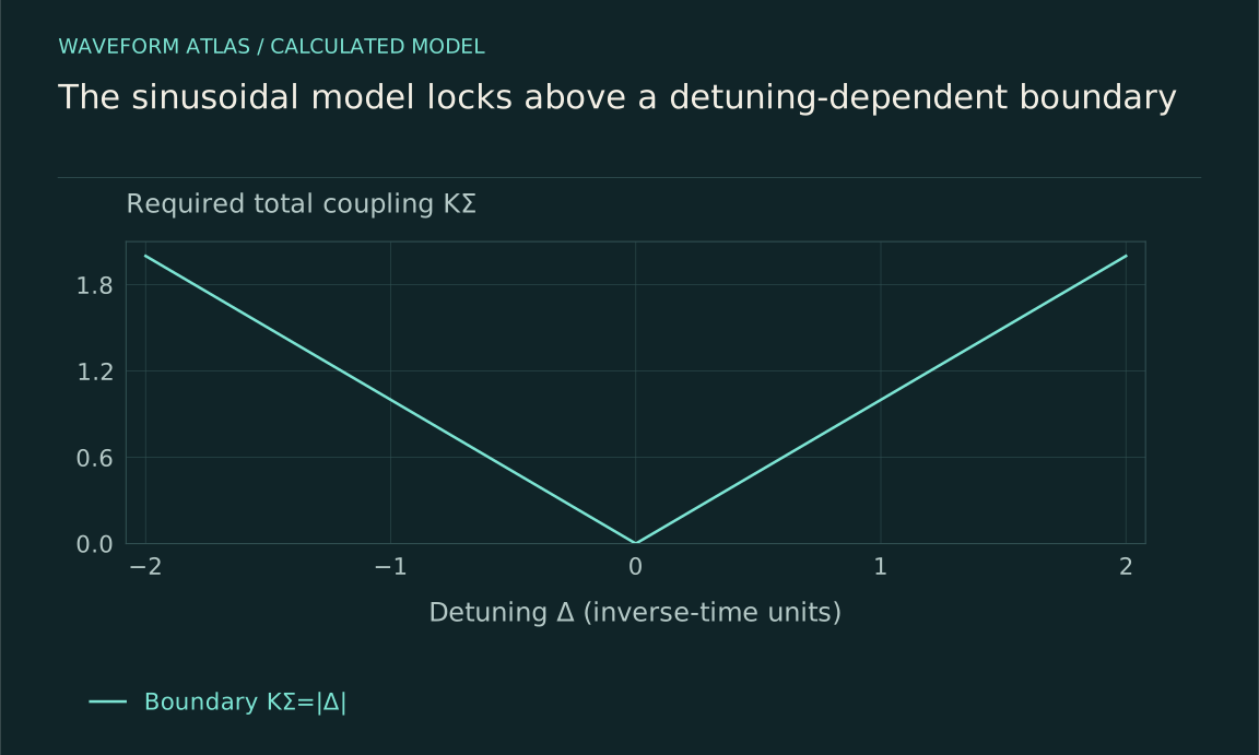
For the sinusoidal model, plotting detuning horizontally and KΣ vertically gives boundaries KΣ=|Δ|. The region widens as coupling increases. In a driven oscillator, related wedge-like regions are often called Arnold tongues, with details depending on the forcing and frequency ratio. The shape is a prediction of a model and chosen coordinates, not a universal drawing that every experiment must reproduce exactly.

Physical actuator strength may not be proportional to KΣ. The conversion depends on phase sensitivity, amplitude and the interaction pathway. Calibrate or infer that relationship before comparing a measured tongue with the simple straight-line boundary. A nonlinear dependence between voltage and effective phase coupling can bend the experimental boundary even when the underlying phase dynamics remain close to the reduced model.

A potential picture explains stable and unstable offsets

The equation φ̇=Δ−KΣsinφ can be written φ̇=−dU/dφ with U(φ)=−Δφ−KΣcosφ. This is a tilted periodic potential for the phase coordinate, not necessarily the literal mechanical energy of the original oscillators. Stable fixed points correspond to local minima and unstable ones to maxima. Increasing detuning tilts the landscape until neighboring extrema disappear.

The picture helps explain why noise can cause slips before the deterministic boundary is crossed: fluctuations can carry the phase over a barrier. It also emphasizes that the phase model is dissipative and reduced. Its potential should not be added to a physical energy ledger without deriving that connection. The actual energy supply and coupling work remain properties of the full oscillator system.

Strong coupling can invalidate phase reduction

A phase-only model assumes amplitude disturbances relax quickly compared with the slow phase adjustment. If coupling becomes strong enough to deform or suppress the oscillation, that assumption fails. Additional states, amplitude dynamics or a full mechanical model may be required. Stronger coupling can also favor antiphase or other patterns rather than simply increasing in-phase alignment.

The metronome studies provide concrete evidence that platform and escapement dynamics affect stable synchronized states. Their relevance is the dependence on the physical interaction, not a universal monotonic rule. Measure amplitudes as coupling changes and check whether the uncoupled cycle remains recognizable. A locking boundary inferred from a weak-coupling model should not be extrapolated indefinitely into a regime with qualitatively different motion.

Delay and phase shifts change the interaction

A delayed coupling signal reaches an oscillator with an additional phase related to the oscillation frequency and travel time. Even if the underlying coupling is simple, the effective phase interaction can acquire a phase shift or memory. The stable offset and locking range then need not match Δ−Ksinφ with a fixed positive K. Multiple stable relations or oscillatory transients can appear in more detailed models.

This is relevant to electrical cables, optical propagation and mechanical support motion. Measure the transfer path and its frequency dependence rather than describing coupling only by a scalar strength. A stronger path with an unfavorable phase can destabilize a desired relation. The interaction's timing is as important as its magnitude when evaluating whether it restores or amplifies a phase error.

Map the boundary with controlled measurements

Measure uncoupled rates, then sweep detuning and coupling while recording both unwrapped phases and amplitudes. Use a stated criterion for locking, such as bounded phase within a window and no resolved slips over a defined duration. Repeat near the boundary because recovery is slow and noise can make outcomes variable. Report finite-time uncertainty rather than drawing an artificially sharp experimental line.

Apply small phase perturbations at selected points and measure recovery. Compare the rate with the model's √(KΣ²−Δ²) prediction when its assumptions hold. Monitor common forcing and changes in source loading. A successful boundary map plus perturbation response provides stronger evidence for the coupling model than a collection of visually aligned traces at favorable settings.

A boundary measurement should also distinguish initial-condition dependence from random failure. If several stable phase relations coexist, the observed state can depend on how the oscillators were started or how coupling was increased. Repeat from different initial phase offsets and record which state is reached. A single successful run does not establish that the desired relation is globally attracting.

The simple sinusoidal two-phase model has one stable and one unstable fixed point per cycle inside its locking range. More complicated coupling functions can have several stable offsets. If the experiment shows reproducible multistability, extend the model rather than forcing every outcome into an unexplained error bar around one predicted phase.

Interpret strength through the observed dynamics

Coupling strength is meaningful only relative to detuning, phase response, amplitude relaxation and noise. In the simple model, the locking inequality and common-frequency formula make those relationships explicit. In a real apparatus, the effective parameters must be connected to the physical interaction and tested over the claimed regime.

The useful conclusion is not that more coupling always produces better synchronization. It is that a specified interaction can compensate a measured mismatch and stabilize a defined phase relation, with quantifiable recovery and slip behavior. That conclusion supports engineering control while leaving energy transfer, amplitude changes, entanglement and other properties to be measured separately rather than inferred from the locking boundary alone.

Go to the original work.

These links identify the sources behind specific claims. Verification scope varies by source and is stated below.

1. 1 / Primary theoryA Study of Locking Phenomena in Oscillators ↗

   Robert Adler. Proceedings of the IRE 34(6), 351–357 (1946).

   DOI: 10.1109/JRPROC.1946.229930

   A reduced phase equation describes injection locking and phase drift under specified oscillator assumptions.

   Verification scope: Publisher or author-institution abstract and bibliographic record inspected; full paper not audited.

2. 2 / Primary theorySynchronization of clocks and metronomes: A perturbation analysis based on multiple timescales ↗

   Guillermo H. Goldsztein; Alice N. Nadeau; Steven H. Strogatz. Chaos 31(2), 023109 (2021).

   DOI: 10.1063/5.0026335

   A model including escapement, amplitude and platform dynamics can have in-phase or antiphase synchronization.

   Verification scope: Publisher or author-institution abstract and bibliographic record inspected; full paper not audited.

3. 3 / Primary theoryHuygens’ Synchronization: Experiments, Modeling, and Local Stability Analysis ↗

   F. N. Hoogeboom; A. Y. Pogromsky; H. Nijmeijer. IFAC-PapersOnLine 48(18), 146–151 (2015).

   DOI: 10.1016/j.ifacol.2015.11.027

   Platform parameters affect the stability of in-phase and antiphase metronome states.

   Verification scope: Publisher or author-institution abstract and bibliographic record inspected; full paper not audited.