Synchronization in a fluctuating environment

A real lock fluctuates

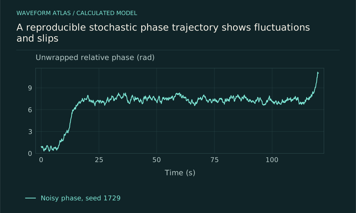
An ideal deterministic phase lock has a stable relative phase. Real oscillators experience fluctuations in frequency, drive, coupling and measurement. The relative phase can wander around its preferred offset and occasionally slip by a full cycle. A practical claim of locking must therefore specify a time interval and an acceptable level of phase variation or slips rather than assuming permanent exact equality.

The source of noise matters. Independent fluctuations tend to disturb the relation differently from fluctuations shared by both oscillators. Measurement noise can also create apparent jumps without changing the physical phases. A useful analysis separates these possibilities through independent references, raw time traces and controlled changes in coupling or environmental inputs.

Define a stochastic phase model

Use dφ=[Δ−Ksinφ]dt+√(2D)dW, where W is a standard Wiener process, K>0 is the effective restoring scale, Δ is detuning and D is a phase-diffusion coefficient. Angles are treated as dimensionless radians, so D has inverse-time units in this convention. The model adds white Gaussian noise to a deterministic Adler-type phase equation.

This is a specific approximation. Colored noise, multiplicative noise, amplitude fluctuations and delayed coupling can require different equations. The noise interpretation must be stated if its coefficient depends on phase; the additive model here avoids that ambiguity. Its predictions illustrate how restoring dynamics and fluctuations compete, but they should not be applied to every oscillator simply because its phase trace looks irregular.

Linearize near a stable offset

When |Δ|<K, the deterministic stable phase satisfies sinφ*=Δ/K. Write ψ=φ−φ* and assume fluctuations are small enough to remain near that point. The linearized equation is dψ=−λψdt+√(2D)dW, with λ=Kcosφ*=√(K²−Δ²). This is an Ornstein–Uhlenbeck approximation for local phase deviations.

Its stationary variance is D/λ and its correlation decays on time scale 1/λ. A stronger restoring rate narrows the local distribution and speeds recovery. Near the deterministic boundary, λ decreases and the same noise produces larger fluctuations. The approximation fails when excursions reach the nonlinear parts of the phase landscape or cross into full-cycle slips, so it is a local description rather than a global locking guarantee.

Calculate a local noise budget

Take K=1 per second and D=0.01 per second. At zero detuning, λ=1 and the rms phase deviation is √0.01=0.1 radians. At Δ=0.8 per second, λ=0.6 and the predicted rms deviation becomes √(0.01/0.6)≈0.129 radians. These are calculated stationary small-fluctuation values for the specified model.

As detuning approaches K, the local variance formula grows without bound, signaling that the approximation is no longer self-consistent. The physical circular phase distribution cannot be described indefinitely by one narrow Gaussian around a fixed point. Use the full stochastic equation or a suitable measured distribution near the boundary. A divergent local estimate is a warning about the approximation, not a prediction of infinite physical phase energy.

A periodic landscape allows slips

The deterministic drift can be written as minus the derivative of U(φ)=−Δφ−Kcosφ. For |Δ|<K, local minima and maxima create barriers in this reduced phase landscape. Noise can carry the phase over a barrier, after which it advances into a neighboring cycle. The unwrapped phase records the slip even though the wrapped angle returns to the same interval.

For positive detuning with r=Δ/K, the forward barrier is ΔU=2K[√(1−r²)−r arccos r]. At zero detuning it is 2K; it decreases toward zero at the deterministic boundary. In a weak-noise regime, escape rates are exponentially sensitive to barrier height divided by D, with prefactors and validity conditions determined by the model. A small parameter change can therefore greatly alter rare-slip behavior.

For K=1 and Δ=0.8 in the stated units, the forward barrier is approximately 0.1704. At D=0.02, the barrier-to-noise ratio is about 8.52, compared with 100 at zero detuning for the same K and D. These ratios illustrate the strong change in rare-event suppression as the locking edge is approached. They are not measured slip rates, and a rate estimate would also need the appropriate prefactor and confirmation of the weak-noise regime.

The reverse barrier differs when detuning tilts the landscape, so positive and negative slips need not occur equally often. A net winding rate can therefore emerge even while the wrapped phase remains concentrated near a preferred value. Measuring both directions helps distinguish biased drift from approximately symmetric phase wandering and provides a sharper test of the proposed stochastic dynamics.

Phase histograms can hide intermittent failure

At Δ=0, the stationary circular distribution for this additive-noise model is proportional to exp[(K/D)cosφ]. It is sharply concentrated when K/D is large and broad when noise dominates. However, a localized wrapped histogram does not reveal how many full cycles the unwrapped phase traversed during the record. Rare slips can coexist with a strongly peaked distribution.

Report both the distribution and the winding history. Count positive and negative slips using a stated criterion, and distinguish net drift from the total number of slips. Equal numbers in opposite directions can give nearly zero mean-frequency difference while still disrupting precise timing. A scalar coherence or order parameter compresses this information and should not replace the time-resolved evidence when reliability matters.

Noise spectra and amplitude zeros complicate phase estimates

White phase noise is a convenient model, but real disturbances often have correlation times or narrow spectral features. Slow frequency drift can move the preferred phase over time, while fast fluctuations broaden it within a short record. Amplitude fluctuations can change the oscillator's instantaneous frequency or make the phase poorly defined near a signal zero.

A numerical phase extractor can then insert a false 2π jump. Check suspicious events against raw waveforms, signal amplitude and an independent reference. Vary filtering and sampling parameters to assess robustness, while avoiding processing that simply removes real slips. The inferred stochastic model should describe the physical timing variable, not artifacts created by the analysis pipeline.

Common noise can coordinate without direct coupling

Teramae and Tanaka showed that common weak additive noise can synchronize a specified class of otherwise uncoupled limit-cycle oscillators. The result is conditional on the oscillator and noise assumptions, not a claim that noise always improves coordination. It demonstrates that correlated motion can have a cause other than direct mutual interaction or a periodic common drive.

This possibility changes experimental controls. Monitor shared environmental fluctuations and, where feasible, vary whether the same disturbance reaches both systems. Compare with independent-noise conditions. If a synchronization claim specifically concerns direct coupling, evidence must distinguish that path from common-noise effects. A high correlation coefficient alone cannot identify which mechanism organized the timing.

Measure a reliability distribution

Acquire records long enough to observe the events relevant to the application, and repeat under controlled conditions. Report phase variance, correlation time, slip count and observation duration rather than only the best interval. If no slips occur, the record supports an upper bound on a rate under a statistical assumption, not proof that the true rate is zero.

Change detuning and coupling to test whether fluctuations and recovery follow the predicted restoring scale. Compare noise spectra or environmental conditions when the model predicts sensitivity to them. A practical locking map can include confidence or reliability contours rather than one sharp deterministic boundary. Such a map communicates how coordination degrades under noise and finite observation, which is often the quantity an engineer actually needs.

If slips are modeled as independent events with a constant Poisson rate λs, observing zero events in duration T gives a one-sided 95-percent upper rate bound of approximately −ln(0.05)/T≈3/T. For T=10,000 seconds, that is about 0.0003 events per second. This is a statistical bound under the Poisson assumption, not a guarantee of future slip-free operation.

Correlated bursts, slow drift or changing operating conditions can invalidate that simple rate model. Retain the timing of all observed events and examine whether intervals are consistent with the assumed process. A long quiet record is informative, but its interpretation depends on stationarity and the event-detection sensitivity. Reporting those assumptions makes a reliability claim more useful than describing the system as perfectly locked.

Interpret noisy coordination without overclaiming

Noise modifies both the dynamics and the evidence available for synchronization. A deterministic stable point can coexist with rare slips, equal mean rates can coexist with phase diffusion, and shared fluctuations can coordinate systems without direct coupling. These are different situations that require different observables and controls.

The useful result states the stochastic model, phase definition, noise source and reliability criterion. It then compares local fluctuations, recovery and slip behavior with predictions over the measured range. This approach treats a lock as a quantifiable dynamical relationship rather than a perfect visual alignment, while keeping energy flow, quantum correlations and collapse claims separate from what the phase statistics establish.

Go to the original work.

These links identify the sources behind specific claims. Verification scope varies by source and is stated below.

1. 1 / Primary theoryAdler (1946), A Study of Locking Phenomena in Oscillators ↗

   A reduced phase equation describes injection locking and phase drift under specified oscillator assumptions.

   Verification scope: IEEE publisher bibliographic record and abstract inspected; the phase equations used here state their own conventions and assumptions.

2. 2 / Primary theoryTeramae and Tanaka (2004), Robustness of the Noise-Induced Phase Synchronization in a General Class of Limit Cycle Oscillators ↗

   Common weak additive noise can synchronize a specified class of otherwise uncoupled limit-cycle oscillators.

   Verification scope: Publisher abstract and author-hosted bibliographic record inspected; scope is the stated oscillator class, not every noisy system.