What synchronization can mean for a quantum system

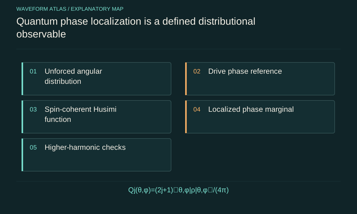
A quantum phase is not automatically a classical trajectory

A classical limit-cycle oscillator can be assigned a position along a repeating orbit when its amplitude remains well defined. A small quantum system is described by a state and measurement probabilities, and it may not support an equally sharp phase variable on each trial. Quantum synchronization therefore requires an operational definition tied to observables rather than an unqualified picture of miniature pendulums.

Possible diagnostics include phase-space localization relative to a drive, correlations between two systems, and changes in spectral or coherence properties under coupling. These are related but not identical criteria. A useful study states which one is measured and what baseline distinguishes the claimed effect from ordinary forced response. The word quantum identifies the system and description; it does not remove the need to define synchronization precisely.

Specify the open-system dynamics

A common framework is a master equation ρ̇=−i[H,ρ]/ℏ+ΣγⱼD[Lⱼ]ρ, where D[L]ρ=LρL†−(L†Lρ+ρL†L)/2. The Hamiltonian contains coherent dynamics and coupling, while the jump operators and rates describe specified dissipative processes. The equation is a model with assumptions about the environment and approximation regime, not a universal form for every possible quantum memory effect.

Gain, loss or engineered relaxation can establish an unforced state with a suitable amplitude or phase-space structure. A weak drive or mutual interaction can then alter its phase distribution or correlations. To claim synchronization, identify that change and its dependence on detuning and coupling. Simply driving a passive quantum oscillator into a coherent response can produce a phase reference without establishing the same autonomous structure as a classical self-sustained cycle.

A phase-space distribution provides one diagnostic

For a bosonic mode, the Husimi function Q(α)=⟨α|ρ|α⟩/π is a nonnegative phase-space representation normalized over the complex plane. A phase marginal can be defined by integrating Q(rexp(iφ))rdr over radius. Its angular structure indicates how the state is distributed relative to the chosen phase reference, subject to the smoothing inherent in this representation.

A ring-like Q distribution can be uniform in angle even when it has a preferred radial scale. A drive can localize the angle. However, a ring-shaped distribution alone does not prove a classical limit cycle: a number state can also have a ring-like Husimi appearance while its dynamics differ from a self-sustained classical oscillator. The state picture must be connected to the actual generator of motion and its response to perturbations.

Finite spins use a different phase space

For a spin j, a spin-coherent-state Husimi function can be written Q(θ,φ)=(2j+1)⟨θ,φ|ρ|θ,φ⟩/(4π), normalized on the sphere. It is not the same function as the planar oscillator Q. An azimuthal marginal can describe localization relative to a drive, while polar structure reflects the finite spin-state geometry. The mapping must be defined before interpreting a plotted angular peak.

For an illustrative spin-1 state |m=0>, this convention gives Q=3sin²θ/(8π), independent of φ. Integrating over polar angle yields a uniform azimuthal distribution. Coherences created by a suitable drive can introduce angular structure. This calculation shows why a finite-level system can support a phase-localization diagnostic without being treated as a classical particle following a sharp orbit at every instant.

For the spin-1 example, the polar normalization can be checked directly: integrating 3sin²θ/(8π) with the solid-angle measure sinθ dθ dφ gives one. The uniform azimuthal marginal is 1/(2π). A phase-localization statistic should therefore compare a driven distribution against that properly normalized baseline, not against a visually chosen flat line with arbitrary scale.

Different phase-space representations can smooth or emphasize different aspects of the same density operator. A change in a plotted distribution is meaningful when the representation and reconstruction are fixed. Comparing numerical peak heights between a planar bosonic Q and a spherical spin Q without accounting for their measures and normalization would be misleading. The state and measured observables, rather than the visual resemblance of two plots, determine the physical comparison.

A verified spin-1 experiment has a specific scope

Laskar and colleagues reported phase synchronization in laser-cooled spin-1 rubidium atoms relative to external classical fields. Their abstract identifies phase-space localization, engineered anisotropic decay and synchronization-related interference features in that setup. The result concerns a particular driven open-system preparation and observable, not a universal claim that all atoms or all resonant transitions synchronize in the same way.

The important methodological lesson is to connect a phase diagnostic with controlled drive and dissipation conditions. A description that mentions only matching frequencies would omit the state preparation and decay structure central to the reported effect. The source has been checked at the publisher-record and abstract level; the explanatory equations elsewhere on this page define their own illustrative models rather than claiming to reproduce the full experimental analysis.

A nuclear-spin experiment uses a measured distribution

Krithika and colleagues studied interacting nuclear spins with an external drive and established phase localization through a measured Husimi distribution. Their abstract also reports detuning-dependent Arnold-tongue behavior and an interferometric method for extracting the distribution. This provides a second concrete example of synchronization being tied to an operational quantum diagnostic rather than inferred from two classical-looking time traces.

The experiment's measurement protocol matters because a reconstructed phase distribution depends on calibrated observables and the assumed state representation. A peak in one plotted distribution should be interpreted within that protocol. It is not automatically a demonstration of entanglement, nor does it imply that a classical phase equation exactly describes every aspect of the finite-spin dynamics.

Quantify localization with the appropriate harmonic

For a normalized phase distribution P(φ), one possible localization measure is C₁=|∫P(φ)exp(iφ)dφ|. It vanishes for a uniform distribution and is large for a narrow single peak. But two equal peaks separated by π can make C₁ vanish despite clear angular structure. A second harmonic or a fuller description of P may be needed for that symmetry.

The choice of measure should follow the proposed synchronization mechanism and reference. A nonzero C₁ can also arise from direct forcing of an otherwise passive system, so compare with an appropriate unforced or uncoupled baseline. No single scalar measure establishes every dynamical feature. Report the distribution, parameter dependence and model alongside the chosen summary statistic.

Relative correlations need not imply entanglement

For two bosonic modes, a normalized correlation such as |⟨a†b⟩|/√(⟨a†a⟩⟨b†b⟩) can quantify a particular first-order phase relation when the denominator is nonzero. Product coherent states with a stable relative phase can make this quantity large. A high value therefore does not by itself prove entanglement or another specifically nonclassical resource.

Conversely, an entangled state need not supply a useful local oscillatory phase or satisfy the chosen synchronization criterion. The two properties concern different aspects of the state and dynamics. If an experiment claims both, it needs both a synchronization diagnostic and an entanglement-sensitive measurement. Treating one as an automatic consequence of the other would erase the distinction that those measurements are designed to test.

Measurement and reference determine what is visible

A phase-sensitive quantum measurement uses a reference and can disturb the system or condition its state. Specify whether results describe an unconditioned density operator, a trajectory conditioned on a measurement record, or selected subsets of trials. Those descriptions can show different apparent phase behavior while remaining consistent with one underlying model. Conditioning should not be hidden inside a claim about the unconditional system.

Calibrate preparation, readout and drive phases, and test whether localization survives reasonable changes in analysis. Monitor population changes and leakage to other levels so that a deformed state is not mistaken for pure timing adjustment. In a finite quantum system, amplitude and phase-like properties can be closely linked. The classical assumption that phase changes independently of a rigid cycle may be only an approximation.

A useful control compares phase localization with changes in the radial or population distribution. If a strong drive simply displaces the state far from its unforced structure, calling the result weak synchronization of that structure may be inappropriate. Scan drive strength and identify the regime in which the intended baseline remains meaningful. The threshold between a useful phase adjustment and substantial state deformation is model dependent and should be established from measured observables rather than from the appearance of a single phase peak.

State the quantum synchronization result operationally

A strong claim names the quantum system, open-system dynamics, reference, measured distribution or correlation, and parameter dependence that establishes the effect. It distinguishes direct drive response from the intended synchronization criterion and reports whether a classical limit is being used for intuition. The verified spin experiments show why those details are substantive rather than optional terminology.

The conclusion need not be universal to be useful. It can establish that a specified quantum observable becomes localized or coordinated under controlled coupling and dissipation. That is distinct from proving entanglement, eliminating fluctuations or demonstrating objective collapse. Keeping those boundaries explicit allows quantum synchronization to be studied on its own measurable terms instead of being forced into an unchanged classical-clock analogy.

Go to the original work.

These links identify the sources behind specific claims. Verification scope varies by source and is stated below.

1. 1 / Primary experimentLaskar et al. (2020), Observation of Quantum Phase Synchronization in Spin-1 Atoms ↗

   A driven, dissipative spin-1 atomic system exhibited phase localization and synchronization-related features.

   Verification scope: Publisher abstract and bibliographic record inspected; no claim of full-paper review.

2. 2 / Primary experimentKrithika et al. (2022), Observation of quantum phase synchronization in a nuclear-spin system ↗

   Driven nuclear-spin phase localization was measured through the Husimi distribution and detuning dependence.

   Verification scope: Publisher abstract and bibliographic record inspected; no claim of full-paper review.

3. 3 / University teachingMIT: Entanglement, Density Matrices, and Decoherence ↗

   Density operators and reduced states distinguish local observables from joint correlations.

   Verification scope: Official university chapter record inspected; elementary examples here are independently worked.