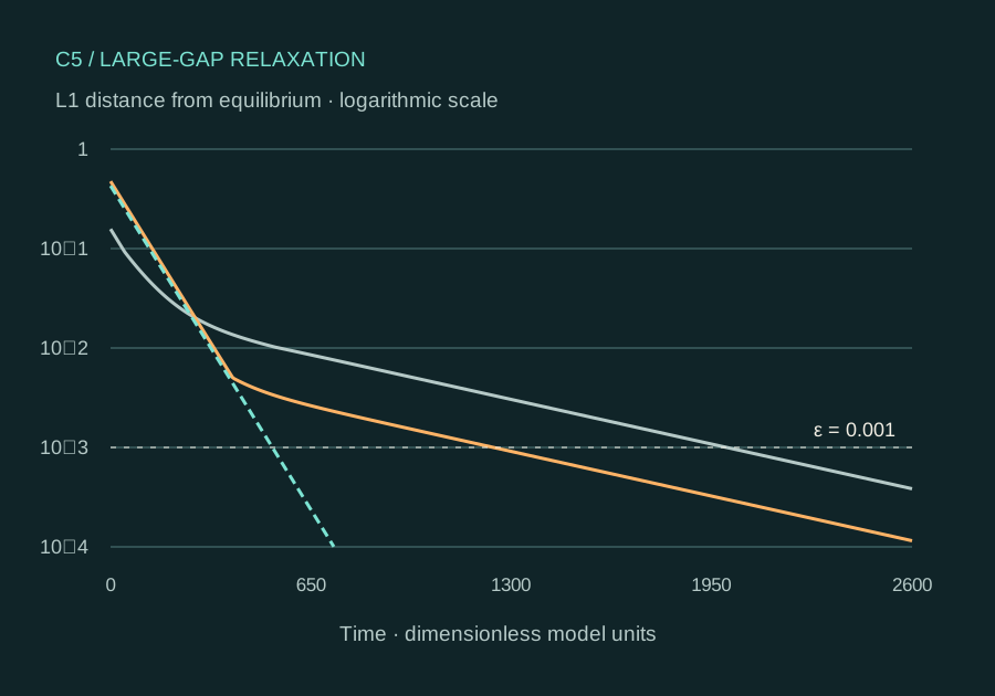
Each comparison holds the generator fixed within its selected fixture. The chosen hot start and the strong-root start are distinct preparations, with different temperatures. Read their labels separately. The graph is a view of the same calculation used by the arrival table.
Faster decay and earlier arrival are different questions
In these detailed-balance chains, the state returns to the same bath equilibrium through two decaying modes. A special initial temperature cancels the slow contribution. That is the asymptotic criterion. An operational comparison asks when the full distribution first reaches a fixed distance from equilibrium.
Klich, Raz, Hirschberg and Vucelja’s work motivates this slow-mode illustration. Our C5 examples were selected from a seeded barrier-model search. They illustrate existence and a distinction between criteria; they do not estimate how common the effect is in nature. Klich et al. · PRX 2019 ↗
C5 / COMPUTED THREE-STATE MODEL
Change the finish line.
Compare the same preparations at a loose or strict distance from equilibrium. The curves and arrival times are computed from the archived three-state generators.
At this threshold, the hot start beats the warm start.
The strong-root preparation arrives even earlier. Change the model and threshold to see where the ordering reverses.
Arrival at the selected threshold · all temperatures and times are model quantities.
Preparation
Initial temperature
Arrival time
Comparison
Warm start
0.494879
1998.331
Reference
Hot start
2.491624
1241.750
Earlier than warm
Strong-root start
1.695126
525.008
Earlier than warm
Slow rate |λ₂| = 0.0015912; fast rate |λ₃| = 0.0115395.
Interactive controls require JavaScript. The reference table and downloadable data remain available.
Equations, units and display limits
dp/dt = Rp, with column sums of R equal to zero. The initial state is a Boltzmann distribution at the selected preparation temperature. L1 = Σ|pᵢ(t) − πᵢ(Tᵦ)|. The browser resolves the two decaying modes algebraically and finds first arrival by bisection.
The vertical axis is logarithmic; values below its lower limit are clipped in the drawing. Table values use the calculation, not a graph reading. kB = 1 and the rate prefactor = 1. These times are not calibrated seconds and these temperatures are not kelvin. Animation speed is only a display control.
Read both criteria
Criterion
What is computed
What it does not establish
Slow-mode cancellation
A nontrivial temperature above the bath with a₂(T) = 0.
The first arrival at every finite threshold, or a universal result for every distance measure.
Finite-threshold arrival
First t with Σ|pᵢ(t) − πᵢ(Tᵦ)| ≤ ε, for the same ε across starts.
A calibrated laboratory time or an energy-saving protocol.
Complete-graph control
Specified uniform-proposal Metropolis rates: no detected nontrivial zero or non-monotone |a₂| in the sampled controls.
A numerical proof, or an exclusion for all complete-graph dynamics.
A reproducible record
2Selected three-state fixtures
500Complete-graph control draws
87 / 87Separate implementation checks
The control draws comprise 300 three-state, 100 four-state and 100 five-state systems. The original C5 rerun reports 11 PASS and 9 INFO. The independent implementation constructs the rates separately and checks a symmetric spectral solution against Radau integration and Poisson uniformization. These are finite numerical checks, not physical experiments.
The separate random-barrier scan detected 13 roots among 300 draws on its specified grid. Sign changes can miss tangential roots and roots outside the interval. The originally unsuccessful hand-picked system is retained as a reconstruction from a source comment; its original failure log was not available.
All trajectories here are nonstationary relaxation transients. They are excluded from the stationary time-shift inference branch. A correct plot does not validate a transient statistical null.
After extracting the bundle, install the pinned dependencies in an isolated Python environment. The wrappers run in temporary working directories and preserve the archived evidence.
The two selected starts called “hot” and “strong-root” have different temperatures. Every table labels them separately. The browser’s algebraic evaluator passed comparisons with 1,806 archived trajectory rows and 30 arrival times. Read the browser validation record ↗
Sources for this chapter
Published work, author attribution and the limits relevant to this chapter. Atlas examples and calculations are labeled separately.