The review sharpened the questions for sensors, resonators, detectors and energy-storage leads. The next advantage must survive a matched component comparison.
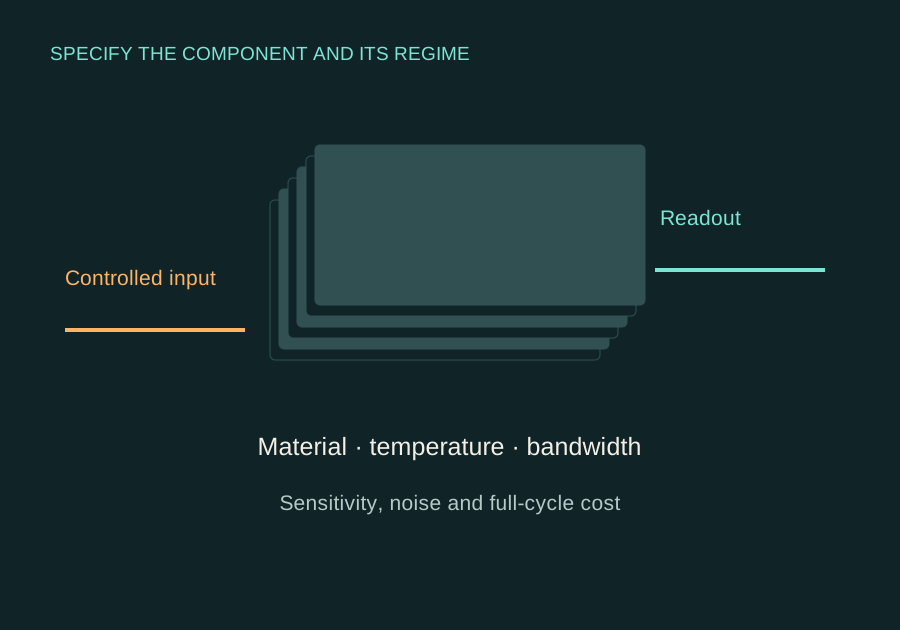
Original conceptual diagram of specimen, controlled input and measured output. It does not depict a fabricated component.
Start with the advantage you can actually measure.
A stronger response becomes useful when it survives the noise, bandwidth and operating conditions of the component.
Suppose two sensors see the same input. One produces twice as much output per unit input. That looks attractive until we ask what happened to output noise, usable range and power. Dividing output noise by response slope gives a simple input-referred noise measure. It lets us compare the input fluctuation that would produce an output of similar size.
That comparison needs matched conditions: bandwidth, averaging, temperature, specimen preparation and calibration. Changing integration time can reduce some noise while hiding a slower response. Changing drive can increase signal while changing heating or nonlinear behavior. A component claim needs the complete operating point.
The candidate has 50% more input-referred noise at these ratios.
Ratio = relative output noise ÷ relative sensitivity. Compare the same bandwidth, integration time, input power, calibration and operating range. This simplified example is not a measured detector specification or a limit of detection.
Work backward from the readout.
WORKED EXAMPLE / ATLAS CALCULATION
A twofold signal gain can give worse input resolution.
Take an illustrative baseline sensitivity of 1 mV per input unit and output rms noise of 0.2 mV. Its input-referred rms noise is 0.2 input units. A candidate with sensitivity 2 mV per unit and noise 0.6 mV gives 0.3 input units. Signal sensitivity doubled, but the input-referred noise grew by 50%.
This is algebra under matched conditions, not a limit-of-detection claim. Detection also needs an error criterion, an estimator and the relevant noise distribution. It shows why a hypothetical response slope cannot decide whether a material class wins.
The same discipline applies to optical collection. More detected light can help, but the comparison must retain spectrum, resolution, dose, collection geometry and fabrication constraints. A useful result names the component and its observable before it is promoted into a system claim.
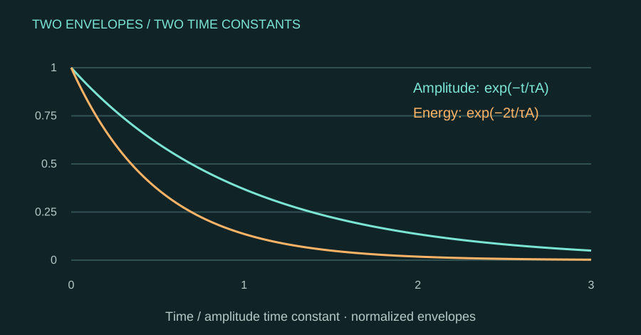
Amplitude decay and energy decay have different clocks.
For an ideal lightly damped linear oscillator, write its amplitude envelope as A(t) = A₀ exp(−t/τA). Energy is proportional to amplitude squared, so the energy envelope decays as exp(−2t/τA). Its e-folding time is τA/2. Confusing those envelopes creates a factor-of-two error.
Calculated normalized amplitude and energy envelopes for a hypothetical linear oscillator. At one amplitude time constant, amplitude is e⁻¹ while energy is e⁻²; these are envelopes, not the oscillating displacement.
WORKED EXAMPLE / ATLAS CALCULATION
Attach the convention to the reported Q.
Under the lightly damped linear approximation, Q ≈ πf₀τA. For a hypothetical f₀ = 1,000 Hz and τA = 0.1 s, Q ≈ 314.2. The energy time constant is 0.05 s; using it in the amplitude formula would halve the answer.
An amplitude-dependent decay need not follow this single exponential. A fitted Q must state the amplitude range, fitting interval, bath conditions and convention. MF-01 therefore retains an amplitude-sweep characterization record. The pattern guides further investigation; it does not pass or fail a proposed athermal mechanism by itself.
For MatterVolt and Lattivara, the next useful step is one accessible specimen and one matched component comparison. For Metric Flight, it is an apparatus-specific loss and noise account. Shared mathematics helps us formulate those comparisons without making their physical systems interchangeable.
Specify the component before claiming the advantage
Question
What changed in the review
Temperature and material
A result in one phase, specimen or cryogenic regime cannot be assigned to another material at product conditions.
Sensor performance
Use the actual response slope, noise spectrum, bandwidth and equal-power comparison. A hypothetical slope cannot settle a whole material class.
Optical performance
Specify wavelength, spectrum, substrate and useful output. Propagation or collection gain is not energy generation.
Detector improvement
Brightness must be read alongside resolution, dose, spectrum, fabrication and the nearest conventional design.
Loss mechanisms
Add the full loss budget; a model of one loss channel is not a measured total quality factor.
Storage claims
Count extraction, retention, preparation and reset costs. A headline charging result does not establish practical system advantage.
Ring-down is characterization
The nanotube simulations are not confined to one 5 K condition. More importantly, ordinary nonlinear damping already makes quality factor amplitude dependent in nanoscale resonators. The revised MF-01 task is to record ring-down against initial amplitude at fixed bath conditions and investigate the pattern. A non-monotonic sweep alone does not select an athermal-mode mechanism. Greaney et al. · nanotube simulations ↗ · Eichler et al. · nonlinear damping ↗
The smallest useful comparison
Choose one accessible specimen, one operating regime and one measurable component outcome. Establish a predictive baseline and a matched fixed alternative. Keep optical, thermal, mechanical and electrical assumptions distinct, then propagate the relevant calibration and specimen uncertainty.
MatterVolt and Lattivara retain their materials investigations. Metric Flight retains its apparatus-specific noise work. These links share a measurement discipline; they do not make the devices or operating conditions interchangeable.
Publication and rights are different records. Identified patent documents remain leads for a claim-specific assessment. No blanket ownership, clearance or “no IP” conclusion is made. Patents for anomalous-relaxation protocols have not been searched.