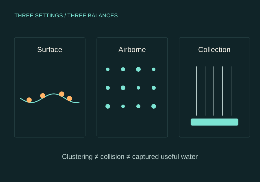
Surface waves, airborne collisions and collection are different stages. A useful transfer has to connect their regimes and measure the final outcome.
Original conceptual schematic: surface floaters, airborne droplets and captured water are shown as different physical settings.
Follow one droplet through the whole question.
A change in the airborne pattern is the start of the investigation. Useful collected water is an endpoint.
A droplet can move with a flow, lag behind it, encounter another droplet, merge, hit a collector, escape, or re-enter the air. A successful intervention must connect the relevant stages. An optical improvement alone does not tell us which pathway occurred.
Two geometries matter immediately: the droplet’s size and the collector’s configuration. Size affects response to a changing flow. Collector geometry affects interception, pressure drop and drainage. Treating either as one nominal number can hide a distribution of outcomes.
TRY THE SCALING / ILLUSTRATIVE INPUTS
Double the radius. Quadruple the response time.
Relative response time
Scale: radius 30 μm at the same fluid properties
Response time τₚ1.235 ms
Stokes number St0.01235
Stokes settling estimate0.0121 m/s
Assumed water density 1,000 kg/m³, air dynamic viscosity 1.8 × 10⁻⁵ Pa·s and g = 9.81 m/s². These are rounded teaching inputs, not measured FogLab conditions. The settling estimate neglects buoyancy relative to droplet weight.
Dilute spherical droplets, continuum Stokes drag and a low particle Reynolds number are assumptions to check. This calculator does not predict a collision kernel, collection yield or outdoor clearing.
A regime map is a comparison of timescales.
For the simplified Stokes-drag calculation, τₚ = 2ρwr²/(9μ). A Stokes number compares this response time with a specified flow timescale: St = τₚ/τflow. With the illustrative values above and τflow = 0.1 s, a 5 μm radius gives τₚ ≈ 0.309 ms and St ≈ 0.00309. A 10 μm radius gives 1.235 ms and 0.01235. The factor of four comes from r².
This calculation is a first coordinate on the regime map. It does not specify the distribution of turbulent velocity gradients, gravity’s role, droplet concentrations, collision efficiency or residence time. Those additional inputs decide whether a collision theory is relevant. A value of St below one is not a fog-clearing prediction.
For a real FogLab comparison, retain the radius distribution and measured flow information, including uncertainty. Evaluate response across that distribution. Document which flow timescale you used; a transit time across the apparatus and a small turbulent timescale are different quantities.
Close the water and power accounts.
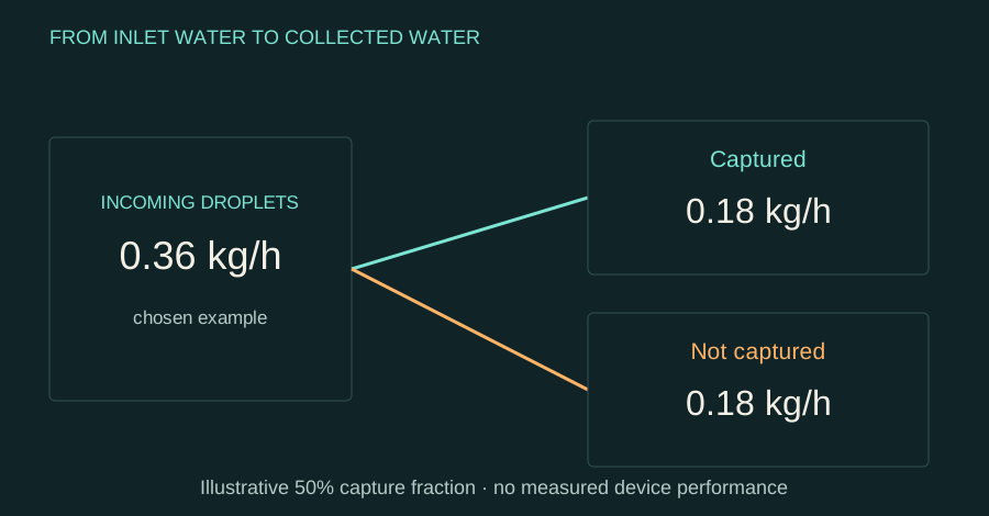
Illustrative collection balance at steady flow: 0.36 kg/h enters as liquid droplets; a chosen 50% capture fraction gives 0.18 kg/h captured and 0.18 kg/h leaving the collection pathway. It is not a measured device result.
WORKED EXAMPLE / ATLAS CALCULATION
An explicit ceiling makes the target clearer.
Assume an air flow of 0.5 m³/s and liquid-water content of 0.2 g/m³. Incoming droplet water is 0.1 g/s, or 0.36 kg/h. At an assumed 50% capture fraction, collected water is 0.18 kg/h. With 60 W of total operating power, the illustrative energy per captured mass is 0.06 kWh / 0.18 kg = 0.333 kWh/kg.
Every number in that example is chosen for teaching. Evaporation, wall storage, leakage, changing inlet conditions and drainage losses must be measured or included in a real balance. If reported collection exceeds the inlet droplet-water estimate, investigate those terms and any additional condensation before attributing a gain to the intervention.
The useful comparison holds flow and inlet conditions fixed, includes all operating power, and records outlet droplets as well as captured water. A contained test can examine that balance without claiming outdoor atmospheric control. The existing Weatherhill and Pluvaryn investigations continue with a more specific endpoint.
Two different particle problems
Vucelja and Fouxon’s 2007 paper concerns particles floating on weak liquid-surface waves. Its growth rate is sixth or higher order in amplitude and too slow on typical natural timescales. It does not supply the missing outdoor airborne-fog scaling. Vucelja & Fouxon · surface waves ↗
The corrected airborne-droplet lead is Falkovich, Fouxon and Stepanov’s cloud-turbulence work. Applying it requires a match to its physical regime, rather than a similarity between two pictures of clustering. Falkovich et al. · cloud turbulence ↗
The regime map we need
Input
Why it matters
Current treatment
Droplet-radius distribution
Response time varies with size; one nominal droplet cannot describe the whole fog.
Retrieve the distribution and uncertainty.
Air properties and velocity gradients
Set droplet response and the relevant turbulent timescale.
Use measured or clearly sourced conditions.
Reynolds number and intermittency
A single Stokes number does not specify the turbulent regime.
Compare the full regime with the theory.
Gravity and settling
Affects transport, collisions and residence time.
Include in the operating envelope.
Collision and collection efficiency
Collision is not the same as captured, useful water.
Measure the pathway to collection.
Define the useful result
Contained collection is a tractable comparison. At matched throughput, record captured mass, droplet escape, pressure drop, total input power and the useful water endpoint. Compare an acoustic approach with appropriate conventional demisting and electrostatic baselines. Ultrasonic demisting study ↗ · Damak & Varanasi · fog collection ↗
Better visibility can result from redistribution without useful capture. Droplet growth can improve one part of the process while increasing losses elsewhere. The next experiment needs a complete balance rather than a single optical trace.
No FogLab operating values are invented here. The regime map is a data requirement. Existing contained-collection and atmospheric investigations remain; this update makes their comparison more specific.