The General Fusion papers connect drive history, compression and diagnostic visibility. Their relevance begins with the apparatus that actually ran.
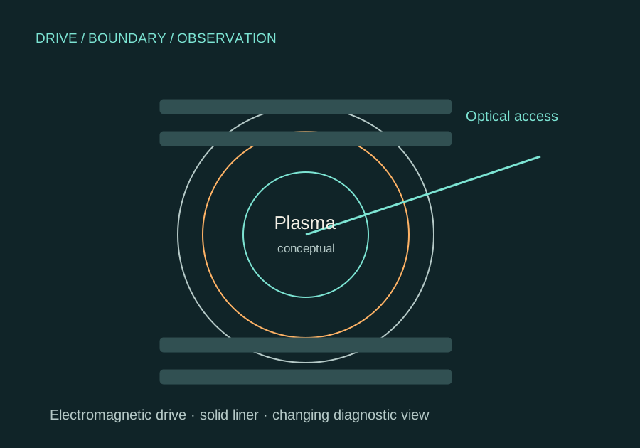
Original conceptual cross-section distinguishing a solid liner, electromagnetic drive and optical access. It is not an engineering drawing or a scaled LM26 reconstruction.
Compression changes more than the radius.
A moving boundary can alter the system’s state and the part of that state an instrument can see.
Start by asking which object moved. Was it a solid liner, a liquid interface, an optical boundary or a wave envelope? The answer determines which conservation laws, material properties and observations belong in the model. The General Fusion lead is useful because it forces these distinctions into the same experimental story.
The next question is how a signal becomes a reported quantity. A measurement samples a place, a time and a response function. If access narrows during compression, later measurements may emphasize a different region. That makes the observation model part of the comparison, alongside the boundary trajectory.
OBSERVATION MODEL / HYPOTHETICAL TWO-ZONE EXAMPLE
The object stays the same. The reading changes.
Keep two hypothetical zones fixed at 1,200 eV and 400 eV. Change only how much weight the readout gives the hotter zone.
1,200 eVFixed hot zone
400 eVFixed cool zone
Weighted readout1,000 eV
Actual zone temperaturesUnchanged
T̃ = w × 1,200 + (1 − w) × 400. At w = 0.25, the same two zones give 600 eV. The apparent decline is entirely an observation-weight change in this toy.
This is an illustrative linear mixture, not a fit to LM26 and not the response function of Thomson scattering, soft X-rays or neutron diagnostics. Real diagnostics require their actual spatial, temporal and spectral response models.
Build the comparison around a measurable bottleneck.
Our transferable question is whether a specified boundary history improves a declared outcome after accounting for observation changes and total control cost. Begin with a fixed reference protocol. Define the same target, tolerances, time horizon and diagnostic model for both candidates. Keep the physical solver, parameter ranges and validation budget visible.
Then separate three costs: finding a protocol, checking it, and executing it. A short final trajectory can be expensive to discover. A cheap approximate solution can need many high-fidelity checks. A protocol that succeeds only under its own fitting assumptions needs a different assessment from one that survives a held-out parameter set.
WORKED EXAMPLE / ATLAS CALCULATION
A successful target can still fail the cost test.
In our recorded inverse-design comparison, both methods reached 24 of 24 tested targets. The proposed search used 470 coarse solves against 270 for the reference. That is (470 − 270) / 270 × 100 = 74.1% more coarse solves, while the declared goal was at least a 20% saving.
This is an accuracy success within the tested cases and a failure of the chosen cost objective. Coarse-solve count is also not a complete wall-clock or energy account. A new methods proposal should retain this result and specify the additional cost measurements it needs.
For Helios, a net-energy claim would need every input, output and reset term over the stated cycle. For Revalith, extraction needs a defined feed, product and regeneration balance. A compression paper supplies neither ledger automatically. The productive connection is a better-defined method question, which can be pursued while hardware holds remain in place.
First separate the machines
System
Actual role
Relevant boundary
LM26
Magnetized plasma compressed with an electromagnetically driven solid lithium liner.
A temperature experiment with changing diagnostic access; not pneumatic pistons compressing molten lithium.
Water-liner study
Pneumatic pistons shape a rotating water liner in a scaled apparatus.
Useful boundary-control research; not a plasma or power-plant demonstration.
Proposed power architecture
A future repetitive fusion plant concept.
Reset, material lifetime, energy balance and useful output remain separate requirements.
Localized measurement shortly before maximum compression.
Electron temperature · filtered soft X-rays
1,180 ± 65 eV
Different time and spatial weighting; not a second value to average with Thomson scattering.
Deuterium-ion temperature · neutron inference
459 ± 33 eV
A different species and inference model.
The October papers were reported as submitted for peer review in the checked records. UKAEA participated in diagnostics and coauthored the work; this is collaboration, not a separate laboratory replication. Raw shot data were not reproduced by the Atlas. LM26 compressional heating study ↗
Geometry changes the experiment and the view
The useful connection is the relationship between a prescribed drive, a moving boundary and what a diagnostic can still observe. In our own control studies, the observation model belongs beside the physical model. An apparent improvement must survive a comparison at matched accuracy and a full account of setup, search and verification cost.
The existing inverse-design branch still failed its cost-saving target: both methods reached the tested targets, while the proposed search used more coarse solves. That failed comparison remains evidence. A new boundary-control example does not erase it.
The next step is a bounded methods comparison. Identify an existing control or diagnostic bottleneck before expanding this lead. These papers supply no new power source for Helios, lithium-recovery chemistry for Revalith, or outdoor-fog scaling for Weatherhill.