Encounter probability is not the same as useful reaction rate

Start with a rate whose units can be audited

For two distinct reacting species, the simplest uniform-plasma expression is R = n₁n₂〈σv〉. Here R counts reactions per unit volume per unit time, n₁ and n₂ are number densities, σ is a reaction cross section and v is relative speed. The angle brackets denote an average over relative velocities. They do not mean that any convenient single speed can replace the distribution.

The units provide a quick consistency check before any numerical substitution or comparison between sources. Each density has units m⁻³. A cross section has units m² and speed has units m/s, so 〈σv〉 has units m³/s. Multiplying gives m⁻³s⁻¹, the required rate density. A formula that produces energy or total counts at this stage has mixed together different quantities.

This expression assumes the relevant pair distribution can be represented by the populations used in the average. Correlations, strongly nonequilibrium beams or spatial structure may need a more detailed treatment. The compact equation is valuable because it makes those assumptions visible, not because every reacting environment must obey the same simplified numerical model.

The average must weight the collisions that actually occur

A cross section is not a geometric ball size. It summarizes the probability of a specified reaction channel for a given incoming state. It can vary strongly with relative energy, and different channels can have different dependence. Multiplying a single tabulated cross section by an average speed can therefore differ substantially from averaging their product.

A simple two-group example demonstrates the issue without pretending to model a real fuel. Suppose 90 percent of pairs have σv equal to one arbitrary unit and 10 percent have σv equal to 30 units. The average is 0.9 × 1 + 0.1 × 30 = 3.9 units. The small high-reactivity group contributes more than three quarters of the total despite containing only one tenth of the pairs.

This is why distribution measurements matter. An inferred temperature may describe a bulk population while missing a tail that dominates reactions. Conversely, a few fast particles do not guarantee a large total yield if their density is extremely small. Rate predictions need the joint weighting of abundance and reaction probability, rather than either feature considered alone.

Work a uniform example without disguising assumed inputs

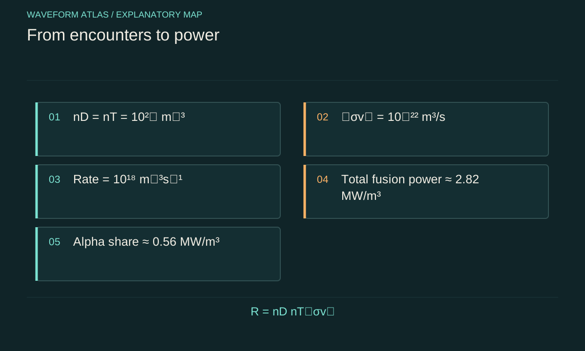
Consider an illustrative D–T mixture with nD = nT = 10²⁰ m⁻³ and an assumed reactivity of 10⁻²² m³/s. Substitution gives R = 10¹⁸ reactions m⁻³s⁻¹. This example specifies reactivity directly; it does not assign a temperature or claim that a particular device achieves it. A real calculation would obtain the value from verified cross-section data and the measured or justified velocity distribution.

Using approximately 17.6 MeV per D–T event, or 2.82 × 10⁻¹² joule, gives total fusion power density near 2.82 MW/m³. A reacting volume of 0.01 m³ maintained for 0.001 second would then produce approximately 10¹³ reactions and 28.2 joules of fusion energy, provided the rate stayed uniform over that interval.

Those conditions matter as much as the arithmetic. A rapidly cooling or expanding plasma will not retain the assumed rate. A hot central region cannot be assigned the entire vessel volume. The example is useful as a dimensional ledger and a scaling exercise; its numbers are not evidence of an experimentally demonstrated source.

Identical reactants require a different pair count

When both reactants are the same species, counting all ordered pairs counts each physical pair twice. The usual dilute-population expression becomes R = ½n²〈σv〉 for a specified identical-species reaction. The one-half factor is combinatorial; it is not a statement that half of the collisions fail. Reaction probability is already contained in the cross section.

A small counting analogy helps. Four distinguishable labeled particles of the same species can form six unordered pairs, not twelve. Pair A–B is the same encounter as pair B–A. For a very large population, N(N−1)/2 approaches N²/2, giving the familiar density factor after the appropriate volume normalization.

Branching introduces a separate factor. If 〈σv〉 represents only one D–D exit channel, the corresponding rate already refers to that exit. If it represents a sum over channels, an additional channel fraction may be needed when predicting one detector’s signal. Applying both a channel-specific cross section and the same branching factor would count the restriction twice. Explicit labels on every input prevent this common bookkeeping error.

Spatial and temporal averaging can change the result

A real source generally requires integration: total yield is the integral of n₁(x,t)n₂(x,t)〈σv〉(x,t) over volume and time. The product must be evaluated before averaging. Multiplying average densities and an average reactivity can miss correlations between hot regions, dense regions and the places where the two fuels overlap.

For example, imagine two equal-sized compartments with the same temperature. One contains only deuterium and the other only tritium, with no mixing. The vessel-averaged densities of both species are nonzero, but their local product is zero everywhere. A calculation using only the vessel averages would predict reactions that cannot occur in that unmixed model.

Less extreme profile effects are often important. A dense cooler edge may contribute less than a smaller hot core, or an energetic beam may react mostly along a narrow trajectory. The appropriate volume is therefore an effective reacting region derived from profiles or diagnostics. Spatially resolved measurements are not merely aesthetic additions to a global yield; they test whether the rate model assigns reactions to physically plausible locations.

A sustained rate consumes and heats its own population

Every D–T reaction consumes one deuteron and one triton. If a uniform source initially contains nD = 10²⁰ m⁻³ and reacts at 10¹⁸ m⁻³s⁻¹ without refueling, its initial fractional deuterium consumption rate is one percent per second. That is an initial slope, not a promise of a constant rate for one hundred seconds, because the reactant densities change as fuel is consumed.

At the same time, charged fusion products can deposit energy and alter the velocity distribution. Transport, radiation and escaping particles remove energy. The coupled evolution can increase or decrease reactivity, so density depletion alone is not enough to predict the time history. Fuel injection and impurity accumulation introduce further population equations.

A steady-state estimate is justified only when these terms approximately balance over the interval being discussed. For a short pulse, an integrated time-dependent calculation may be more appropriate. The distinction between an instantaneous peak rate and total yield is particularly important: a spectacular peak sustained briefly can produce less total energy than a moderate rate maintained much longer.

Confinement changes the opportunity to react

The rate equation is local and instantaneous. Confinement enters by determining how long a population with particular density and energy remains available. Particle confinement and energy confinement are related operational concepts but are not identical. A plasma may retain many particles while losing their thermal energy rapidly, which changes the reaction probability even before the particles leave.

A simple survival picture gives another useful limit. If a tagged deuteron encounters a fixed tritium population with constant effective reaction frequency λ = nT〈σv〉, its probability of reacting within time t is 1 − exp(−λt), assuming independent encounters and no competing processes. For λt much smaller than one, this reduces to λt. A longer residence time then increases the chance roughly linearly.

That model becomes inadequate if the particle slows, heats, escapes or sees a changing target density. It nevertheless separates the probability for one particle from the total rate generated by many particles. Confinement is valuable because it preserves favorable conditions; it is not an additional nuclear reaction channel or a substitute for a sufficient cross section.

Close the calculation with measured products and boundaries

An experimentally useful rate estimate predicts recorded products. Start with the channel-specific yield, then apply emission geometry, transport through surrounding material, detector efficiency, timing and analysis selection. Comparing the result with data tests both the plasma model and the measurement model. Disagreement should be traced to a specific term rather than hidden inside a general correction factor.

Power requires another explicit step: multiply each reaction-channel rate by its released energy and identify where that energy goes. Total D–T fusion power includes neutron energy that does not directly heat a magnetically confined plasma. The alpha component is much smaller and is the relevant starting point for a self-heating balance. Electrical output introduces still more conversion and operating losses.

A credible rate statement therefore names its density convention, distribution assumption, reaction channel, spatial boundary and time interval. These details make different experiments comparable. They also explain why demonstrating some fusion events, demonstrating a large instantaneous rate and demonstrating a useful sustained energy source are separate achievements requiring different measurements.

Go to the original work.

These links identify the sources behind specific claims. Verification scope varies by source and is stated below.

1. 1 / University teachingRichard Fitzpatrick: Lawson Criterion ↗

   Rate nD nT〈σv〉, energy-confinement time W/Ploss and an explicitly idealized self-heating balance.

   Verification scope: University page, assumptions and displayed equations inspected.

2. 2 / University teachingRichard Fitzpatrick: Nuclear Fusion Reactions ↗

   D–T reaction kinematics, product energy partition and distinct charged-particle/neutron energy channels.

   Verification scope: University teaching page and displayed equations inspected; broad introductory approximations retained only with explicit limits.

3. 3 / Official researchITER: The magic cocktail of deuterium and tritium ↗

   ITER: The magic cocktail of deuterium and tritium. https://www.iter.org/node/20687/magic-cocktail-deuterium-and-tritium

   The D–T reaction releases approximately 17.6 MeV; the article compares fusion cross sections for different fuels and temperature regimes.

   Verification scope: Official ITER explanation inspected; used for total D–T energy and fuel/temperature context, not a derivation of velocity-distribution averaging.

4. 4 / University teachingStructure and Evolution of Stars, Lecture 10: Thermonuclear Reactions ↗

   University of Cambridge. Structure and Evolution of Stars, Lecture 10: Thermonuclear Reactions (2017), slides 5–15.

   Coulomb repulsion, relative collision energies, thermally averaged reaction rates and the competition of tunneling and thermal factors at the Gamow peak.

   Verification scope: University lecture slides 5–15 inspected. This introductory source does not calibrate the atlas illustrative reactivity to a device or temperature.