Larger motion can lead to nonlinear failure

Large amplitude can invalidate a linear model

Linear wave theory assumes disturbances are small enough that the governing response can be approximated around a background state. Under that approximation, wave speed and superposition are independent of amplitude. As disturbances grow, neglected nonlinear terms can become important. Different parts of the waveform may then travel differently or interact with one another.

This does not imply that every amplified wave must break. Some systems saturate, form stable nonlinear waves, transfer energy into other modes, or remain within a useful weakly nonlinear regime. The relevant measure can be steepness, strain, intensity, or displacement relative to a background scale, not amplitude alone. A water-wave height relative to wavelength and depth conveys more than height by itself. An optical intensity requires a material response and interaction length to predict nonlinear change. The model and its dimensionless parameters define the boundary.

Amplitude-dependent speed produces steepening

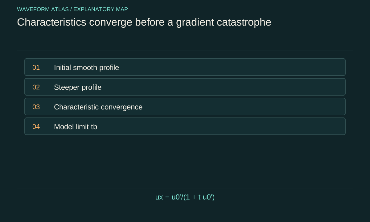
A simple scalar model is ut+c(u)ux = 0. The local value u travels along a characteristic whose speed is c(u). If higher values move faster and lie behind lower values, the rear can catch up with the front. The profile becomes steeper even if its maximum value remains bounded.

This geometric mechanism is easier to see than a generic claim that the wave becomes too large. It depends on both the amplitude-dependent speed and the initial slope. A profile with the opposite slope can spread instead of steepen. The same model can therefore produce compression or rarefaction from different initial conditions. Rodolfo Rosales's university materials treat characteristics and nonlinear kinematic wave breaking as a model-analysis problem, emphasizing that a failed smooth solution signals the need to include additional physical structure rather than a failure of conservation itself.

An explicit breaking-time calculation

For inviscid Burgers' equation ut+uux = 0, characteristics satisfy x = ξ+u0(ξ)t and u = u0(ξ), where ξ labels the initial position. Differentiating gives ux = u0′(ξ)/[1+t u0′(ξ)]. If the initial derivative is negative somewhere, the denominator first reaches zero at tb = −1/min u0′.

For the illustrative initial profile u0(x) = A sin(kx), the most negative derivative is −Ak, so tb = 1/(Ak). With A = 1 meter per second and k = 2π inverse meters, tb is about 0.159 second. The amplitude remains bounded while the slope diverges in the ideal smooth model. This is a gradient catastrophe, not an infinite energy or infinite amplitude prediction. The example shows why increasing amplitude or shortening wavelength can bring nonlinear steepening forward in time under the specified equation.

Crossing characteristics mark a description limit

After the predicted breaking time, the naive characteristic construction can assign several values of u to the same position and time. For a single-valued fluid or traffic density variable, that is not an acceptable physical continuation. The model must be interpreted with shocks, dispersion, viscosity, or more detailed dynamics appropriate to the system.

The mathematical singularity therefore identifies where an approximation or smooth-solution assumption fails. It does not establish that the underlying physical system ceases to exist. A numerical simulation can hide this issue if its discretization adds artificial smoothing. Conversely, an unstable numerical method can create apparent blow-up that the physical equation does not predict. Resolution studies, conservation checks, and a known analytical limit help distinguish physical steepening from numerical artifacts. The article's Burgers example is deliberately a model calculation, not a universal quantitative forecast for ocean waves or optical pulses.

Shocks enforce a conservation account

For a conservation law ut+∂xF(u) = 0, a discontinuity moving at speed s satisfies the Rankine–Hugoniot relation s = [F(uL)−F(uR)]/(uL−uR), provided the states differ. For Burgers' flux F(u) = u²/2, this gives s = (uL+uR)/2. Additional admissibility conditions select physically relevant shocks rather than every formal discontinuity.

With illustrative left and right values 3 and 1 meters per second, the shock speed in that model is 2 meters per second. The jump condition expresses conservation of the modeled quantity across the moving front. It does not mean every other quantity, including mechanical energy, is conserved by an inviscid discontinuous idealization in the same way. Dissipative physics can convert organized motion into heat. The appropriate conserved variables and entropy condition depend on the actual physical equations being modeled.

Viscosity and dispersion regularize differently

Adding viscosity to Burgers' equation gives ut+uux = νuxx. The diffusive term smooths steep gradients over a finite scale and dissipates the model's quadratic energy under appropriate boundary conditions. Adding dispersion instead can produce oscillatory structures that redistribute phase and energy without the same local dissipative mechanism.

These outcomes are not interchangeable. A smooth shock-like front, an oscillatory dispersive wave train, and a physically overturning water surface may look like related failures of a sinusoid but require different equations. The dominant balance among nonlinearity, dispersion, and dissipation determines the relevant scale. Measuring only the disappearance of the original waveform cannot identify which balance occurred. Spatially resolved profiles, spectra, and energy or heat measurements can help. A model should include the mechanism that actually arrests steepening rather than simply labeling its unresolved endpoint collapse.

Fluid breaking adds geometry and turbulence

A surface water wave can overturn, entrain air, and generate turbulent motion. That physical breaking process involves a moving free surface and multiple spatial scales, beyond the one-dimensional scalar example. Organized wave energy can become currents, vortices, smaller waves, sound, and eventually heat. A lower coherent wave amplitude after breaking is therefore part of an energy redistribution.

Thresholds depend on water depth, wave shape, currents, focusing, and other conditions. A single universal maximum amplitude would ignore those dependencies. Linear dispersion relations remain useful reference points but cannot describe the entire breaking event. Measurements of surface elevation alone may miss subsurface kinetic energy and turbulent dissipation. The term breaking is appropriate when tied to a defined observable such as overturning or a validated steepness criterion for a stated regime, rather than used as a metaphor for every large-wave change.

An amplifier can trigger a nonlinear regime without defining it

An active source can increase a wave until nonlinear propagation matters. The amplifier supplies energy; the medium then determines how that larger wave evolves. Gain saturation in the source and wave breaking in the propagation medium are separate mechanisms, even when both limit the observed amplitude.

To distinguish them, measure the waveform immediately after the amplifier and again after propagation. If distortion is already present at the source, amplifier nonlinearity may dominate. If it develops with distance while the source output remains stable, nonlinear propagation is implicated. Varying medium length, background conditions, or wavelength provides additional tests. A large local peak can also arise from passive focusing or interference without active gain. The energy source and the route to steepening should be identified separately before assigning the observed failure to amplification itself.

What to measure near the onset

Record spatial or temporal profiles with enough resolution to capture growing gradients, and monitor spectra for harmonics or broadband redistribution. Measure input energy and relevant output channels. Repeat across amplitude, wavelength, and propagation distance to test the predicted scaling. For the Burgers example, the product Ak sets the inverse breaking time, giving a specific model prediction to compare with controlled data.

Instrument bandwidth can smooth the very gradients of interest, while aliasing can create false oscillations. Calibration and numerical processing therefore belong in the interpretation. If a simulation is used, demonstrate convergence and check its handling of conservation and dissipation. A visually dramatic waveform is not enough to establish a singularity or a new physical law. The strongest evidence connects a measured trend to a stated equation and identifies where that equation's assumptions cease to be adequate.

Breaking is not quantum-state collapse

A nonlinear wave can lose its original coherent shape through steepening, mode transfer, turbulence, or dissipation. These are statements about classical fields or collective variables under specified dynamics. Quantum-state collapse concerns a different set of questions about measurement updates or proposed fundamental modifications of quantum evolution.

The shared word collapse can obscure the distinction. A gradient becoming large in an approximate equation does not show that a quantum superposition has objectively reduced, and a broken water wave does not imply energy annihilation. The useful conclusion is that larger amplitude can expose nonlinear physics omitted from a small-signal model. Identify that physics, follow the energy, and measure the new scales that appear. This approach turns wave breaking into a concrete dynamical subject without treating every loss of a familiar waveform as the same phenomenon.

A conservation audit should use the quantity actually conserved by the model. The integral of u in a scalar conservation law is not automatically the physical energy of a water wave. Translating model variables back to density, momentum, surface elevation, or field amplitude is necessary before claiming that a numerical invariant closes the experimental energy budget.

Go to the original work.

These links identify the sources behind specific claims. Verification scope varies by source and is stated below.

1. 1 / University teachingWave Propagation — Triantaphyllos Akylas, lecture notes ↗

   Triantaphyllos Akylas. Wave Propagation — Triantaphyllos Akylas, lecture notes. 2017.

   Transient wave propagation, elastic modes, interfaces and water waves

   Verification scope: Official chapter contents and author-written course records inspected

2. 2 / University teachingRodolfo Rosales — Principles of Applied Mathematics lecture summaries ↗

   Rodolfo Rosales. Rodolfo Rosales — Principles of Applied Mathematics lecture summaries. 2014.

   Characteristics, nonlinear wave steepening, shock conditions and regularization

   Verification scope: Official author course page and linked topic summaries inspected; used for model scope

3. 3 / University teachingFundamentals of Photonics: Quantum Electronics — lecture notes ↗

   Franz X. Kärtner. Fundamentals of Photonics: Quantum Electronics — lecture notes. 2006.

   Population dynamics, absorption/gain, Rabi oscillations and coupled modes

   Verification scope: Official author-written course materials and topic mapping inspected

4. 4 / University teachingSignals and Systems — Alan V. Oppenheim, lecture notes ↗

   Alan V. Oppenheim. Signals and Systems — Alan V. Oppenheim, lecture notes. 2011.

   Convolution, linear systems, filtering and feedback

   Verification scope: Official course notes and topic records inspected

5. 5 / University teachingQuantum Optical Communication — Jeffrey H. Shapiro, readings and lecture slides ↗

   Jeffrey H. Shapiro. Quantum Optical Communication — Jeffrey H. Shapiro, readings and lecture slides. 2016.

   Author-written quantum attenuator, amplifier, detection and parametric interaction framework

   Verification scope: Official course materials and topic mapping inspected

6. 6 / Primary researchBreaking Waves in Deep and Intermediate Waters ↗

   M. Perlin; W. Choi; Z. Tian. Annual Review of Fluid Mechanics 45, 115–145 (2013).

   DOI: 10.1146/annurev-fluid-011212-140721

   Surface-wave breaking geometry, onset criteria and energy dissipation; review concerns deep and intermediate water depths.

   Verification scope: Publisher bibliographic record and abstract inspected; full review not reread