A wave can change the form in which it travels

A mode is a specified pattern of motion or field

A mode is a solution pattern appropriate to a system's geometry, material properties, and boundary conditions. It can specify a spatial profile, polarization, frequency, propagation direction, and normalization. In a waveguide, modes can have distinct transverse shapes and propagation constants. In an elastic solid, longitudinal and shear modes involve different directions of material displacement.

Calling a process conversion requires identifying which mode was occupied initially and which modes carry the output. A detector that sees only the input mode can report a loss even when energy has moved coherently into an orthogonal mode. Conversely, changing the mathematical basis used to describe an unchanged field is not necessarily a physical conversion. The definition should be tied to fixed preparation and analysis procedures. This turns the statement that the wave changed form into a measurable input-output relation.

Several distinct properties can be converted

Polarization conversion changes the relative amplitudes and phases of vector-field components. Spatial-mode conversion changes the transverse pattern. Elastic mode conversion can transfer energy between longitudinal and shear motion. Frequency conversion changes the oscillation frequency through an appropriate interaction. A device can perform more than one of these operations simultaneously.

These categories have different energy and symmetry implications. A static lossless waveplate can change polarization at the same frequency without supplying net optical energy. A pump-driven frequency converter can raise a photon's frequency by supplying the energy difference. An elastic interface can split one incident wave into several reflected and transmitted modes at the same frequency. Grouping all of these as wave collapse hides the mechanisms. The useful comparison is which mode labels change, which remain conserved, and which external degrees of freedom participate.

Coupling requires an interaction with the right structure

Two modes do not exchange energy merely because they have been named. A perturbation or interaction must connect their field patterns. In a coupled-waveguide model, overlap between fields and the altered dielectric structure produces coupling. At an elastic boundary, continuity conditions generally require a combination of modes. In a nonlinear optical medium, a pump can create a polarization source at a new frequency.

Symmetry can make a coupling vanish even when modes occupy the same region. For example, an overlap integral can cancel between positive and negative parts of an odd pattern when the perturbation is symmetric. Breaking that symmetry can enable transfer. Phase mismatch can also suppress accumulation despite nonzero local coupling. A converter therefore needs more than proximity or a large material response: it needs spatial overlap, compatible symmetry, and the appropriate phase and frequency relations over the interaction region.

A two-mode model shows reversible transfer

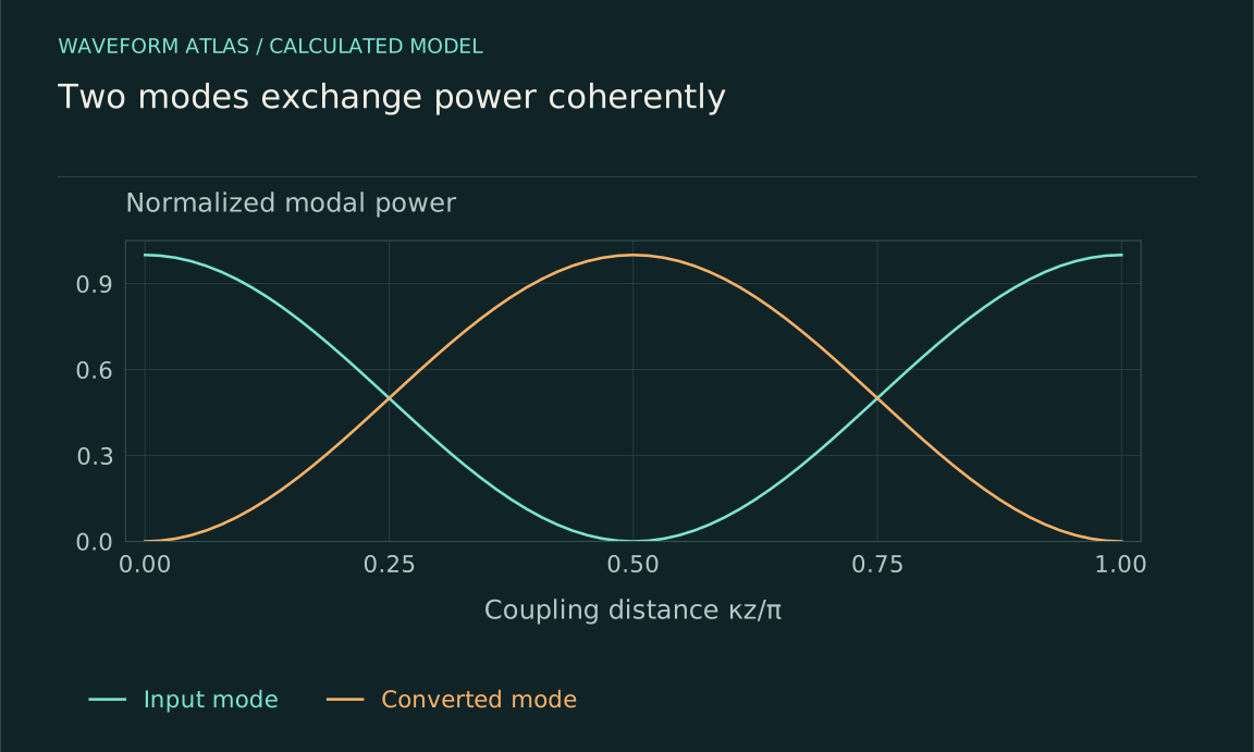
For two lossless, equally normalized modes with constant real coupling κ and no mismatch, a simple propagation model is i da1/dz = κa2 and i da2/dz = κa1. With a1(0)=1 and a2(0)=0, the solution gives modal powers |a1|² = cos²(κz) and |a2|² = sin²(κz). Their sum remains one.

At κL = π/2, the input is fully transferred to the second mode in this ideal model. At κL = π, it returns to the first with a phase change. More interaction length does not therefore always mean more useful conversion. The oscillation is coherent exchange, not irreversible loss. Real devices include mismatch, radiation, absorption, and additional modes, which alter the result. The model is valuable because it provides a concrete baseline against which those effects can be measured rather than inferred from a fading input-mode signal alone.

Power normalization prevents a false budget

A mode amplitude must be related to energy or power using the appropriate normalization. Equal displacement amplitudes in longitudinal and shear waves do not necessarily carry equal power because their speeds and impedances differ. Equal optical field amplitudes in modes with different cross sections also need not carry equal total power.

For a passive, stationary, lossless converter with all propagating outputs included, total outgoing power equals incoming power in a steady-state account. In a pulse experiment, include temporary stored energy and integrate over the full output. A pump-driven device adds a pump term, and a moving or time-varying medium can exchange work with the field. The same energy conservation principle applies, but the ledger changes. Reporting a squared amplitude ratio as efficiency without checking normalization can make a perfectly ordinary converter appear to create or destroy energy.

Frequency conversion needs a photon-energy distinction

For narrowband optical modes, photon flux is power divided by ℏω. An ideal converter that maps one input photon to one higher-frequency output photon preserves photon number in that selected conversion while increasing signal power. The extra energy comes from the pump. A down-converter can reduce signal power while still converting every input photon into the desired lower-frequency mode.

For an illustrative doubling of frequency with unit photon-number conversion, output signal power is twice input signal power. Calling that a 200-percent efficiency without stating the denominator is misleading. It is a power ratio for a pumped process, not a wall-plug energy efficiency. The pump and any companion modes complete the budget. This distinction is central when comparing classical conversion measurements with quantum interfaces, where preservation of a single excitation and its encoded state may matter more than raw output power.

Coherence can survive a change of mode

A deterministic lossless mode transformation can preserve relative phases and quantum superpositions. A photon encoded in a temporal or polarization superposition can, under an appropriate converter, emerge at a different frequency while retaining the encoded coherence. That possibility must be tested with interference or state-sensitive measurements, not inferred from conversion counts alone.

Primary frequency-conversion experiments have demonstrated specific quantum-interface and time-bin coherence results under their device conditions. Those results establish that conversion need not be inherently decohering; they do not guarantee perfect fidelity for every mode or operating point. Pump phase noise, loss, unwanted emission, and mode-dependent efficiency can degrade the output. Separate the probability of obtaining the desired output from the quality of its conditional state. A converter can have high conditional fidelity but low total success probability, or high power transfer with substantial added noise.

A gradual converter follows changing eigenmodes

Some devices change their structure gradually so that an input follows an evolving local eigenmode. The mode can begin concentrated in one guide or polarization and end in another. This adiabatic strategy differs from stopping a uniform coupler at one precisely chosen exchange length.

The relevant condition is that structural variation is slow compared with the separation and coupling of local modes. Near a small eigenvalue gap, a change that is gentle by geometric appearance may still be too rapid dynamically. A longer device can improve following but also accumulate absorption, scattering, or fabrication errors. Adiabatic does not mean automatically lossless or independent of wavelength. A useful design compares nonadiabatic transfer into unwanted modes with ordinary propagation loss and the required bandwidth. The local eigenmode picture explains the intended mechanism, while measurement determines whether it is actually followed.

Mode-resolved detection distinguishes conversion from filtering

Measure the input and several output modes with calibrated analyzers. A polarization analyzer, spatial-mode projector, spectral filter, or elastic displacement measurement selects different properties. Confirm that the desired output appears with the expected dependence on coupling, pump, geometry, or phase, and account for residual input and other channels.

A filter can make the surviving output look purer by discarding unwanted modes without converting them. A pump can generate background in the desired output band even with no input. A finite detector aperture can mistake beam reshaping for loss. Controls with the input blocked, pump changed, analyzer rotated, or converter detuned help distinguish these possibilities. A successful conversion claim should identify a transfer relation, not merely a preferred-looking output image. Total throughput, modal purity, and noise should be reported separately.

A practical receiver can define useful conversion more tightly than a camera does. Suppose a beam transmits eighty percent of its incident power, but only half of that transmitted field power overlaps the receiver's accepted mode. The delivered target power is forty percent of the input. Enlarging the camera's collection area may increase measured throughput without changing this delivered fraction. The receiver's mode definition therefore belongs in the conversion specification from the start.

The wave changes its carrier pattern, not into nothing

Mode conversion is a concrete route by which an initially recognizable wave becomes less visible in one channel and more visible in another. It can be passive or driven, coherent or noisy, nearly reversible or accompanied by dissipation. The classification depends on the measured dynamics rather than on the disappearance of the input pattern.

The most useful account names the modes, coupling mechanism, phase conditions, energy source if any, and measurement basis. It then quantifies useful output, residual input, parasitic channels, and uncertainty. Those details connect optical, acoustic, elastic, and quantum examples without pretending they are identical. A converted mode is evidence of redistribution or driven transfer within a larger system. It is not, by itself, evidence that energy vanished or that a fundamental wavefunction-collapse law acted.

Go to the original work.

These links identify the sources behind specific claims. Verification scope varies by source and is stated below.

1. 1 / University teachingWave Propagation — Triantaphyllos Akylas, lecture notes ↗

   Transient wave propagation, elastic modes, interfaces and water waves

   Verification scope: Official chapter contents and author-written course records inspected

2. 2 / University teachingFranz Kärtner — Classical Electromagnetism and Optics, chapter 2 ↗

   Coupled-mode equations, power normalization, polarization and waveplate transformations

   Verification scope: Official author PDF selected sections 2.7 and 2.9 equations inspected; not all 159 pages read

3. 3 / University teachingWave Propagation, chapter 3: Two Dimensional Waves — MIT course notes ↗

   Elastic P/SV/SH modes, planar boundary matching, mode conversion and critical angles

   Verification scope: Official chapter outline and selected boundary equations inspected; PDF text extraction is partly garbled

4. 4 / University teachingFundamentals of Photonics: Quantum Electronics — lecture notes ↗

   Population dynamics, absorption/gain, Rabi oscillations and coupled modes

   Verification scope: Official author-written course materials and topic mapping inspected

5. 5 / University teachingElectromagnetics and Applications — lecture notes ↗

   Poynting theorem, boundary conditions, material response and polarization

   Verification scope: Official author-written course and topic records inspected

6. 6 / University teachingQuantum Optical Communication — Jeffrey H. Shapiro, readings and lecture slides ↗

   Author-written quantum attenuator, amplifier, detection and parametric interaction framework

   Verification scope: Official course materials and topic mapping inspected

7. 7 / Primary experimentA photonic quantum information interface — Tanzilli et al. (2005) ↗

   An optical up-conversion interface tested preservation of quantum correlations

   Verification scope: Author preprint abstract inspected; historical device-specific performance

8. 8 / Primary experimentCoherent frequency-down-conversion interface for quantum repeaters — Curtz et al. (2010) ↗

   Difference-frequency conversion of weak time-bin states with interference verification

   Verification scope: Author preprint abstract inspected; pseudo-single-photon input scope retained

9. 9 / University teachingQuantum Physics III — Adiabatic theorem and Landau-Zener lectures, MIT ↗

   Instantaneous eigenstates, adiabatic approximation and nonadiabatic transitions

   Verification scope: Official course lecture-topic record inspected; explicit two-mode calculations in articles are original worked models