Longitudinal and shear waves at an interface

Longitudinal and shear modes move material differently

In an isotropic homogeneous elastic solid, a longitudinal or P wave has displacement parallel to its propagation direction. A shear or S wave has displacement perpendicular to propagation. The two wave types have different speeds determined by density and elastic moduli. Their energy fluxes and boundary stresses therefore differ even at the same frequency.

For a planar two-dimensional incidence problem, shear motion is often separated into SV, polarized in the plane of incidence, and SH, polarized perpendicular to that plane. These labels refer to geometry, not different fundamental particles. In a simple isotropic planar setting, P and SV can couple through the boundary conditions, while SH forms a separate problem. Anisotropy, roughness, or three-dimensional geometry can change that separation. A conversion diagram should state the assumed material symmetry and coordinate plane before drawing every shear polarization as interchangeable.

The boundary must satisfy more than a displacement picture

At a perfectly bonded interface between ideal elastic solids, displacement continuity and traction continuity constrain the total fields. Traction is the force per area exerted across the interface and includes normal and tangential components. An incident P wave alone generally cannot satisfy all conditions at oblique incidence, so reflected and transmitted P and SV components are needed.

The coefficients follow from solving the coupled boundary equations with the material parameters and allowed propagation directions. A sketch that simply rotates the displacement arrow does not determine those coefficients. At a free surface, traction vanishes instead of matching another solid. At an ideal fluid–solid boundary, the fluid does not support an ordinary propagating bulk shear wave and the tangential condition differs. These are distinct physical problems. The correct boundary model is the mechanism that enables or restricts conversion.

Frequency stays fixed at a stationary interface

For a linear interface that does not change in time, every participating harmonic field has the same frequency as the incident wave. The wave number magnitude changes because P and S speeds differ. The boundary can therefore change wavelength and polarization without changing temporal frequency.

A moving or explicitly time-dependent interface can exchange energy and produce frequency shifts, but that is outside the stationary model. This distinction prevents elastic mode conversion from being confused with generic frequency mixing. A time-domain pulse contains many frequencies, each with its own conversion coefficients and delays. The output can be reshaped even though each frequency component obeys the stationary matching rule. A broadband measurement should therefore account for frequency-dependent conversion rather than assume one angle and one amplitude coefficient describe the entire pulse.

Tangential phase matching determines the angles

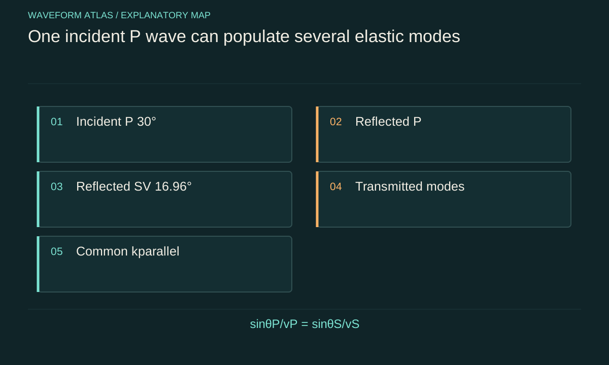
Along a uniform planar interface, the phase variation must agree for all coupled waves. Thus the tangential wave number kparallel is common. With angles measured from the normal and k = ω/v, the relation is sinθ/v = constant for the participating propagating modes. This is the elastic counterpart of Snell's law.

For an illustrative incident P wave in a solid with vP = 6,000 meters per second and vS = 3,500 meters per second, at θP = 30 degrees, a reflected SV component in the same solid satisfies sinθS = (vS/vP)sinθP = 0.2917. Its angle is about 16.96 degrees from the normal. This calculation fixes a possible direction, not its amplitude. Boundary stresses and the properties of the other side determine how much energy enters that mode. Phase matching and conversion strength are separate parts of the problem.

Normal incidence can forbid conversion by symmetry

For an ideal isotropic planar interface at normal incidence, a longitudinal wave produces no preferred tangential direction, and the usual P-to-SV conversion vanishes. A shear wave can likewise obey a decoupled symmetry class. Oblique incidence breaks the simple normal-incidence geometry and allows the coupled traction conditions to generate another polarization.

The statement is conditional on the interface and material assumptions. An anisotropic crystal, textured surface, finite beam, or structured layer can introduce additional coupling. Observing conversion near nominal normal incidence may therefore reveal misalignment or a departure from the ideal model rather than a violation of elastic theory. A useful control scans the angle through zero and compares the symmetry of the response. The measured angular dependence can test both the proposed coupling mechanism and the alignment of the source and detector.

Amplitude ratios are not energy fractions

For a plane harmonic elastic wave with peak displacement amplitude A in an isotropic medium, a useful flux scale is one half ρω²v|A|² along its propagation direction. The component crossing a planar interface includes a cosine of the propagation angle. P and S modes have different v and may occupy media with different density.

Consequently, the squared displacement-amplitude ratio of a converted wave is not generally its power conversion efficiency. The appropriate flux factors must be included. In a lossless interface problem with all propagating channels accounted for, reflected and transmitted power fractions sum to one. An illustrative ledger with fractions 0.20, 0.15, 0.40, and 0.25 in reflected P, reflected S, transmitted P, and transmitted S closes the budget, but it is not a solved boundary-condition result for the earlier speed example. Labeling such examples prevents a bookkeeping illustration from becoming fabricated experimental data.

Critical angles change which modes propagate

If the phase-matching relation requires |sinθ| greater than one for a candidate mode, that mode has no ordinary real propagation angle in the bulk. Its normal wave-number component becomes imaginary, producing an evanescent field under the relevant branch choice. The boundary can still require that field to satisfy local conditions.

A single evanescent component in a lossless semi-infinite medium does not carry the same far-field normal power as a propagating transmitted wave. Finite layers, coupled interfaces, or dissipation can create more complicated energy transfer, so evanescence should not be equated with no physical effect. Near a critical angle, amplitudes and phases can vary sharply, and finite beam width matters. A detector designed only for propagating bulk modes can miss near-interface energy or surface-wave coupling. The measured channel set should match the regime being tested.

For a concrete limit, let an incident SV wave in a solid have speed 3500 m/s and its converted reflected P wave have speed 6000 m/s. Tangential matching requires sin θP = (6000/3500) sin θSV. A propagating reflected P ray exists only up to θSV = arcsin(3500/6000), approximately 35.7 degrees from the normal. Beyond that angle the P contribution must be treated as evanescent in the normal direction; drawing a real outgoing P ray would violate the dispersion relation.

Pulses separate modes through travel time and polarization

Because P and S speeds differ, converted pulses can arrive at different times along known paths. Their displacement directions provide another distinguishing observable. A receiver sensitive to one component may strongly favor one mode and underreport another, making receiver calibration part of the conversion measurement.

For equal ten-millimeter propagation lengths at the illustrative speeds 6,000 and 3,500 meters per second, travel times are about 1.67 and 2.86 microseconds. The difference is about 1.19 microseconds before accounting for actual ray geometry. A pulse shorter than that scale may help resolve the arrivals, but its bandwidth can encounter varying conversion coefficients and dispersion. A complete interpretation combines timing, polarization, and geometry rather than assigning every later pulse to a converted mode. Reflections from other boundaries can produce similar delays.

An experiment should test the boundary model

Prepare a known incident polarization and scan incidence angle or frequency. Measure reflected and transmitted displacement components, calibrate receiver sensitivity, and convert amplitudes into fluxes with the appropriate speeds, densities, and angles. Compare the results with a boundary-condition calculation using independently measured material parameters where possible.

Control surface roughness, bonding quality, finite beam size, and sample geometry. A poorly bonded interface may support slip or extra loss, invalidating a perfect-bond model. Multiple reflections in a finite sample can interfere with the primary converted wave. Time gating can help separate paths, but the gate itself must not discard a significant part of the desired pulse. Report residual input mode, converted modes, and unexplained loss separately. Agreement across several observables is stronger evidence for mode conversion than a single reduced transmitted amplitude.

Conversion preserves a larger mechanical account

The incident wave can leave energy in longitudinal motion, shear motion, reflected paths, surface modes, or dissipative channels. The original displacement pattern may become weak at one receiver while other modes carry substantial energy. This is a redistribution determined by material response and geometry, not disappearance of mechanical energy.

The simple planar isotropic model offers clear predictions about frequency, tangential phase, and allowed polarizations. Departures from those assumptions should be investigated through the additional physics they introduce. Elastic mode conversion is therefore both a useful engineering mechanism and a diagnostic of interfaces. It does not require a universal collapse threshold or a particle-annihilation analogy. A precise account follows the displacement and stress fields into all relevant modes and tests their flux balance under stated experimental conditions.

Go to the original work.

These links identify the sources behind specific claims. Verification scope varies by source and is stated below.

1. 1 / University teachingWave Propagation, chapter 3: Two Dimensional Waves — MIT course notes ↗

   Elastic P/SV/SH modes, planar boundary matching, mode conversion and critical angles

   Verification scope: Official chapter outline and selected boundary equations inspected; PDF text extraction is partly garbled

2. 2 / University teachingWave Propagation — Triantaphyllos Akylas, lecture notes ↗

   Triantaphyllos Akylas. Wave Propagation — Triantaphyllos Akylas, lecture notes. 2017.

   Transient wave propagation, elastic modes, interfaces and water waves

   Verification scope: Official chapter contents and author-written course records inspected

3. 3 / University teachingSignals and Systems — Alan V. Oppenheim, lecture notes ↗

   Alan V. Oppenheim. Signals and Systems — Alan V. Oppenheim, lecture notes. 2011.

   Convolution, linear systems, filtering and feedback

   Verification scope: Official course notes and topic records inspected