Reading an angular scattering pattern

Treat the pattern as a directional measurement

An angular scattering plot is a map of signal versus outgoing direction. For a three-dimensional experiment, a direction generally needs two angles. A line scan through one plane is only a slice of that map. The distinction matters when an object is asymmetric or when polarization selects a preferred direction. A beautiful polar curve can conceal large regions that were never measured.

Begin by defining the incident direction, the target orientation and the detector's angular resolution. State whether the radial coordinate represents field amplitude, intensity, counts, probability density or a differential cross section. These quantities have different units and cannot be compared just because their plots share a shape. The detector may also integrate over frequency, polarization or target motion. Those integrations belong in the definition of the observable. A faithful figure makes the experimental choices visible before suggesting what the pattern reveals about the target.

Path differences turn geometry into fringes

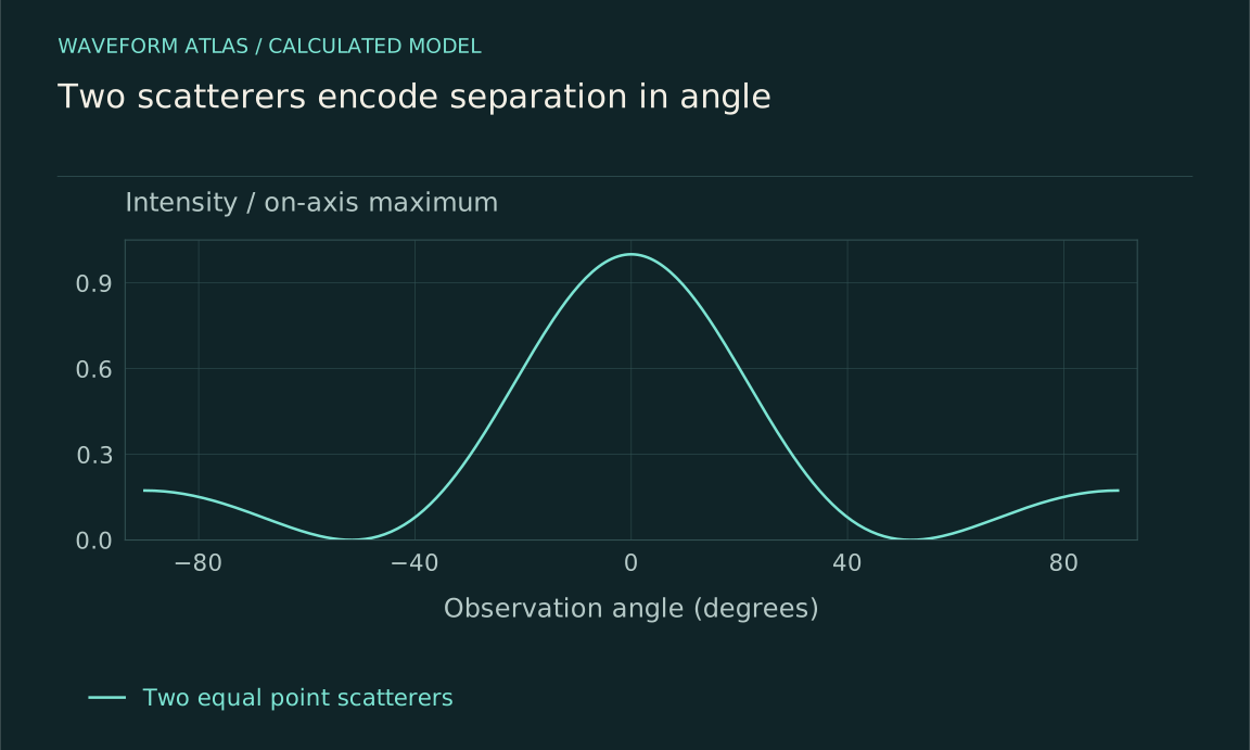
Consider two ideal identical point scatterers separated by a vector d. In a simple single-scattering model, their contributions differ in phase by q·d, where q is the change in wavevector between incident and detected directions. If each contributes the same amplitude f, the total amplitude is f[1 + exp(iq·d)]. The intensity is proportional to 2|f|²[1 + cos(q·d)]. Geometry appears through a phase difference, not through an extra source of energy.

The assumptions are substantial: identical response, stable separation, coherent illumination and negligible repeated scattering between the objects. Within those limits, changing d changes fringe spacing, while changing the single-object response f changes the envelope. This separation is useful because it distinguishes information about arrangement from information about individual scatterers. In a real specimen the two effects can be coupled, and a model that treats them as independent must justify that approximation over the measured wavelength and angular range.

An illustrative two-scatterer example

Choose a geometry in which q·d = kd sin θ and k = 2π/λ. If d = 2λ, the relative phase is 4π sin θ. The first positive-angle destructive minimum occurs when that phase reaches π, giving sin θ = 1/4 and θ approximately 14.5 degrees. If the separation doubles to 4λ, the corresponding minimum moves to approximately 7.2 degrees. The numbers follow from the stated ideal geometry; they are not fitted to experimental points.

This example explains why finer angular features can accompany larger structures. It also shows the danger of inverting one minimum mechanically. A different orientation, unequal amplitudes, a phase offset between scatterers or a nontrivial single-scatterer envelope can shift or fill the minimum. A reliable inference should predict several features across the pattern and survive a change in wavelength. A single dark angle is a clue, not a complete structural reconstruction. The experimental task is to make competing explanations produce measurably different predictions.

The envelope describes the individual response

Even before several scatterers interfere, one extended object can have a structured angular response. Contributions from different parts of that object acquire different phases. Material resonances and boundary conditions determine their relative strength. The resulting envelope may be broad, sharply forward directed or strongly dependent on polarization. It need not resemble the object's outline.

The ratio of object size to wavelength is a useful organizing parameter. When the size is small compared with wavelength, a low-order response can dominate. As more spatial variation fits across the object, additional angular structure becomes possible. This is a guide to model selection rather than a universal recipe. Shape, contrast and absorption matter as well. An inverse calculation should therefore state which parameters were allowed to vary. If a fit assumes a sphere, it has found a sphere compatible with the data, not proved that no nonspherical target could produce a similar measured pattern.

Symmetry helps only when the apparatus respects it

A symmetric target often produces related angular features, but the incoming field and measurement geometry can break the apparent symmetry. Polarization selects a direction. An oblique beam distinguishes one side from another. A detector with uneven sensitivity can create an apparent preferred angle. Before attributing an asymmetric lobe to new target physics, rotate the target and separately rotate or recalibrate the detection arrangement.

A target-fixed feature follows the target under controlled rotation; an apparatus-fixed artifact tends to remain associated with the instrument. This diagnostic is not perfect when illumination changes during rotation, so monitor the input beam and keep the illuminated region registered. Sample mounting can also strain or shadow the object. Record these details rather than assuming that rotation changes only orientation. Symmetry is powerful because it generates testable relationships among data, but it is strongest when those relationships are checked across multiple configurations instead of inferred from one aesthetically symmetric image.

Averaging can erase useful structure

If scatterers move or the illumination loses coherence over the relevant path differences, interference features can wash out in an averaged intensity pattern. That smoothing does not necessarily mean each individual realization lacked interference. A camera can integrate many different speckle patterns into a smooth halo. The exposure time and the target's correlation time therefore affect what information survives in the displayed figure.

Compare short and long acquisitions when practical, and distinguish an ensemble average from a single stable realization. Spectral bandwidth can produce similar smoothing because different wavelengths place fringes at different angles. Angular resolution also fills narrow minima by averaging over nearby bright directions. A broad observed feature may consequently reflect the source or detector rather than the target. The model-to-data comparison should include these averaging operations explicitly. Otherwise a loss of contrast can be misidentified as a material property or as an irreversible loss of coherence in the underlying dynamics.

Intensity alone leaves phase ambiguity

Most ordinary detectors measure an intensity or count rate, which depends on the squared magnitude of an amplitude. The phase of that amplitude is not directly recorded. Different complex fields can therefore share the same angular intensity. This is one reason structural inversion can be nonunique even with an accurate detector and an excellent signal-to-noise ratio.

Additional information can reduce the ambiguity: a known reference field, several incident angles, wavelength variation, polarization analysis or prior constraints on the target. Each addition should be justified by the question being asked. A phase-sensitive measurement can reveal information unavailable in intensity alone, while a strong structural prior can make a limited dataset useful at the cost of model dependence. Report both the recovered parameters and the alternatives the measurement cannot distinguish. The honest inverse problem is not weakened by showing uncertainty; it becomes more useful because readers know which features are supported by data and which were supplied by assumptions.

Design the next angular measurement

Choose the angular range and resolution from the scale of the feature you want to discriminate. A narrow predicted minimum requires sufficient angular sampling and a detector aperture small enough to resolve it. Measure backgrounds with the target absent and with the source blocked. Normalize by a monitored incoming flux so a drifting source cannot masquerade as a changing scattering strength.

Then test the structural explanation with a control that changes its phase prediction. Wavelength variation is often especially informative because geometric path differences scale with k. Orientation changes can distinguish symmetry classes, and polarization can probe directional response. Fit all relevant configurations together rather than adjusting a separate model to every image. The result should connect a measured pattern to a constrained physical description, with uncertainties and missing angles visible. That is how an angular plot becomes evidence about structure instead of a decorative picture of where light happened to appear.

Finite apertures blur sharp predictions

A calculated angular pattern usually describes an ideal point detector in the far field. A real detector integrates over a finite angular interval. Its recorded value is an average of the differential signal weighted by the acceptance function, not the theoretical curve evaluated at the center angle. A narrow minimum can consequently appear filled even when the underlying fields cancel exactly at one direction.

For the two-scatterer example, increasing separation makes fringes narrower. A camera with fixed angular pixel width can therefore show lower measured contrast for the more widely separated pair. This does not demonstrate a loss of coherence. It may mean that each pixel sums neighboring bright and dark directions. Reducing the aperture, increasing the observation distance while preserving angular calibration, or modeling the instrument response can distinguish these possibilities.

The far-field approximation itself needs checking. It replaces spherical propagation from different parts of an object with a direction-dependent phase factor. Close to an extended object, curvature matters and the pattern changes with observation distance. An apparent departure from a far-field formula may thus be an ordinary near-field effect. Record sample size, wavelength, detector distance and aperture alongside the plotted angles. These quantities make the result reproducible and identify whether disagreement belongs to the scatterer, to the approximation, or to how the scattered field was sampled.

Go to the original work.

These links identify the sources behind specific claims. Verification scope varies by source and is stated below.

1. 1 / University teachingQuantum Physics III: Scattering and Identical Particles ↗

   Scattering states, differential cross sections, phase shifts and their assumptions.

   Verification scope: MIT course page and lecture topic descriptions inspected; this is a teaching reference, not a new experiment.

2. 2 / University teachingMIT Physics III: Vibrations and Waves ↗

   Wave equations, interfaces, optics and propagation in media.

   Verification scope: MIT course outline inspected; article derivations are independent textbook-level explanations.

3. 3 / Primary experimentVellekoop and Mosk, Focusing coherent light through opaque strongly scattering media ↗

   The reported control of incident wavefronts to focus transmitted multiply scattered light.

   Verification scope: University author-repository abstract and publication metadata inspected; no claim of a full-paper methods audit.