What decoherence explains in a measurement

Begin with a system and an environment

A quantum system is rarely isolated from every surrounding degree of freedom. Light, gas, support structures and internal modes can become correlated with its alternatives. Decoherence studies how these correlations affect the interference available in measurements on the system alone. The environment need not be consciously observed. It matters because it physically carries information and because the experiment typically does not control or measure all of it.

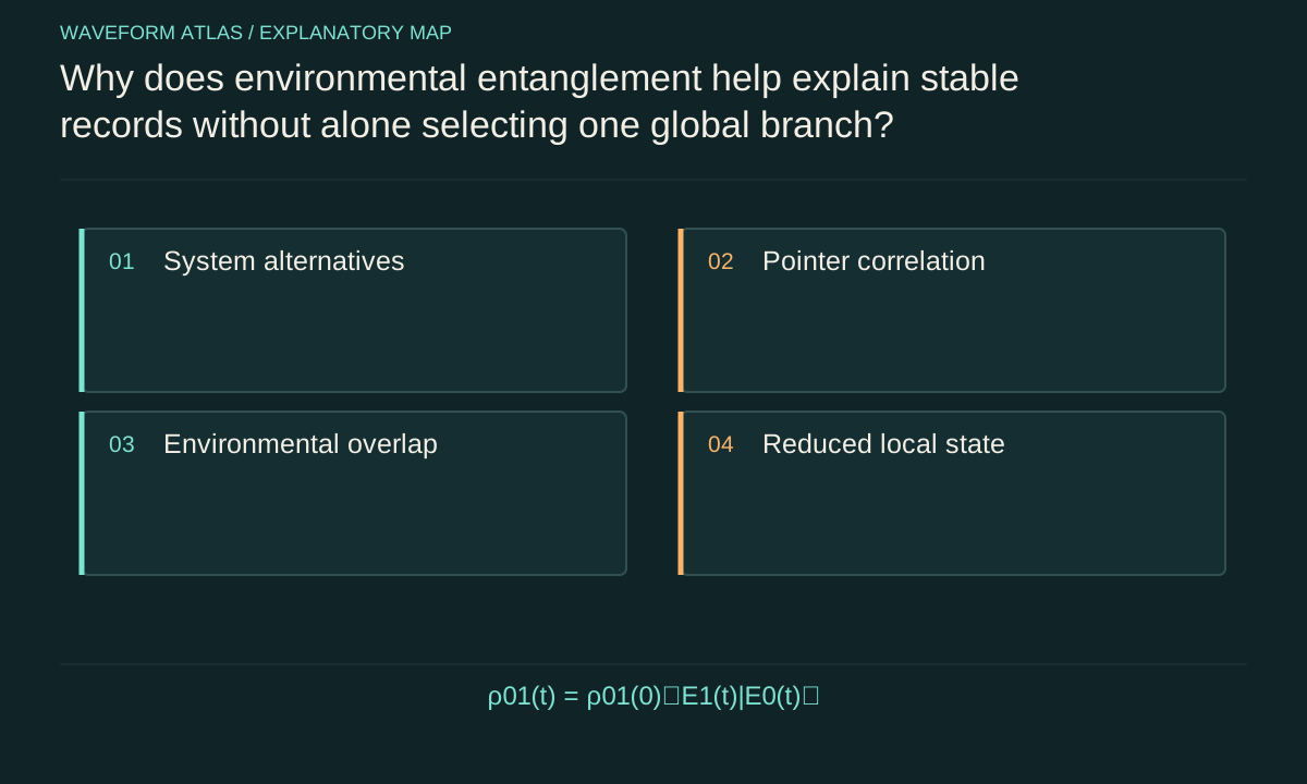
Consider a superposition a|0⟩ + b|1⟩ interacting with an initially uncorrelated environment. A simple interaction produces a|0,E0⟩ + b|1,E1⟩. The environmental states depend on the system alternative. The local state is obtained by tracing over the environment. This calculation connects an explicit interaction to observable statistics, rather than invoking a vague idea that complexity automatically destroys quantum behavior.

Derive the interference factor

The reduced density matrix has diagonal entries |a|² and |b|² and off-diagonal entry ab*⟨E1|E0⟩. If the environment states are identical, their overlap has magnitude one and the local coherence is preserved up to a phase. If they are orthogonal, the off-diagonal entry vanishes. Intermediate overlap produces partial suppression. The environmental record’s distinguishability controls the local interference in this idealized model.

The populations can remain unchanged while coherence decreases. This is why decoherence should not automatically be described as energy loss. A system may retain the same probability of occupying each energy level while losing a phase relation between them. Other interactions cause both relaxation and dephasing. The terms should follow the actual observables and coupling, not be used interchangeably whenever a signal becomes smaller.

Compare a mixture with an entangled state

For an equal superposition and orthogonal environment records, the local state is an equal mixture of zero and one. The same local density matrix could arise from a classical random preparation that selected zero or one in advance. Local measurements alone cannot distinguish these cases. The distinction lies in the joint correlations: the entangled preparation can be globally pure, while the classical mixture has a different joint state.

This is sometimes expressed by distinguishing an improper mixture from an ignorance mixture. The terminology is less important than the calculation. Tracing out a subsystem yields the correct local probabilities, but it does not assert that the whole state physically became one term. A global measurement or reversal could in principle reveal coherence if all relevant degrees of freedom were controllable. In realistic macroscopic settings, that control can be overwhelmingly difficult without being ruled out by the unitary model itself.

Explain why some records are robust

Different system observables couple differently to the environment. States that remain relatively stable under the dominant interaction can form a preferred set of records, often called pointer states. A position-sensitive environment, for example, can rapidly distinguish sufficiently separated locations. The resulting local dynamics suppress interference between those alternatives more strongly than between alternatives the environment cannot distinguish.

This mechanism helps explain why everyday records have an approximately classical structure rather than appearing in arbitrary superpositions. It does not mean the preferred basis is universal or independent of the apparatus. Change the coupling and the stable states can change. A careful account derives the relevant basis from the interaction and timescales. Simply declaring that position is always classical would miss systems where another observable is monitored or where coherent control protects different degrees of freedom.

Work a visibility example

Take equal path amplitudes and an environmental overlap γ. In an ideal balanced recombination measurement, the output probability can be written p(φ) = [1 + Re(γe^{iφ})]/2. If γ is real and positive, the fringe visibility is γ. An overlap of 0.8 yields maxima and minima of 0.9 and 0.1; an overlap of zero yields a flat one-half distribution. These numbers are calculated for a simple two-path model.

A real visibility measurement also depends on path imbalance, detector response and phase stability. If one path is attenuated, the maximum achievable contrast can change even without the same kind of environmental record. If the phase drifts between trials, averaging can suppress fringes. The environmental-overlap model is therefore a mechanism to test, not a universal interpretation of every low-contrast pattern. Additional controls are needed to identify which contribution dominates.

Distinguish decoherence from classical phase averaging

A random classical phase applied to a system can produce the same reduced dephasing channel as entanglement with an unobserved environment under suitable conditions. From system-only data, these descriptions may be indistinguishable. Access to the noise record or environment can change what recovery is possible. If the phase is known, an inverse rotation may restore coherence. If information is dispersed into inaccessible modes, recovery is much harder.

This does not make the reduced description wrong. It means that one channel can summarize several physical situations at the level of the observed subsystem. To identify a mechanism, measure additional correlations or vary the suspected noise source. A fitted dephasing rate is a useful operational quantity, but it is not automatically a unique microscopic explanation. The same caution applies when a new collapse model predicts a similar decay of off-diagonal elements.

State what decoherence does not settle alone

Under a purely unitary system–environment description, the global state retains correlated alternatives. Decoherence explains why their interference is locally inaccessible and why certain records behave robustly. By itself, the partial-trace calculation does not choose one global branch as the unique outcome. Different interpretations explain the relation between the global state and definite records in different ways, while objective-collapse theories alter the dynamics.

This limitation should not be used to dismiss decoherence as irrelevant. It solves concrete physical problems about interference, information transfer and record stability. Nor should its success be used to declare every foundational question solved without stating an interpretation. The productive position is precise: decoherence provides a mechanism with measurable consequences, and the account of a single outcome may require additional interpretive or dynamical commitments depending on the framework adopted.

Compare with objective-collapse predictions

A collapse model can add suppression of coherence beyond the environmental channels predicted by standard quantum theory. To test it, one must calculate the additional effect and distinguish it from ordinary interactions. Mass dependence, separation dependence, duration, temperature and secondary heating or radiation may provide discriminating features. A disappearing off-diagonal element alone is not enough because conventional open-system dynamics can produce the same local signature.

The baseline environmental model should be constrained independently where possible. Otherwise a free fitted decoherence rate can absorb either technical noise or a proposed new contribution without identifying either one. If the models remain observationally equivalent for the chosen protocol, the experiment cannot decide between them. A second observable or a changed control parameter is then more useful than stronger language about what the first curve supposedly proves.

Recovery tests reveal accessible information

An echo sequence can reverse certain forms of phase dispersion, and a controlled interaction can sometimes undo entanglement with a small auxiliary system. Successful recovery shows that the relevant coherence was not irretrievably removed within the tested model and control range. It can help distinguish reversible inhomogeneous broadening from other processes. The interpretation depends on exactly which couplings the reversal addresses.

Failure to recover does not by itself prove fundamental irreversibility. The inverse operation may be inaccurate, the environment may contain uncontrolled records or the system may have undergone energy relaxation. Recovery is therefore a diagnostic with asymmetric implications: success can rule out some claims of irreversible destruction, while failure leaves several explanations. A useful experiment quantifies control fidelity and tests known reversible cases before drawing conclusions from an unsuccessful reversal.

Make the explanatory boundary useful

A strong decoherence account identifies the system, environment, interaction, relevant overlap or channel and measured observable. It predicts how coherence changes under controlled variations and explains which records become stable. It then states whether the global dynamics are assumed unitary and what additional interpretation is used for individual outcomes. This structure makes the physical explanation and the foundational commitments visible separately.

For measurement, decoherence is therefore neither a synonym for every collapse nor an optional decorative detail. It is the physical study of how correlations with unobserved degrees of freedom change accessible interference. That role is essential to understanding real apparatus, while its limits keep the measurement problem sharply posed. Readers can use the distinction to evaluate both conventional detector models and proposals for new dynamics without treating every lost fringe as the same phenomenon.

A useful reporting convention separates the observed contrast from the inferred coherence factor. The former comes directly from counts after response correction; the latter requires assumptions about balance, reference noise and the recombination instrument. Showing both makes it easier to see which conclusions are data driven and which depend on the chosen physical model. It also makes later reanalysis possible when a better model becomes available.

Go to the original work.

These links identify the sources behind specific claims. Verification scope varies by source and is stated below.

1. 1 / Primary theoryDecoherence, einselection, and the quantum origins of the classical ↗

   Wojciech H. Zurek. Reviews of Modern Physics 75, 715 (2003). Linked record is the author preprint.

   DOI: 10.1103/RevModPhys.75.715

   Environmental monitoring, preferred records and suppression of local interference.

   Verification scope: Author-posted review abstract and APS bibliographic record inspected; source supports the decoherence framework, not an independent audit of each apparatus or biological state.

2. 2 / University teachingPreskill, Quantum Information, Chapter 2: States and Ensembles ↗

   Preskill, J. Quantum Information, Chapter 2: States and Ensembles. Caltech lecture notes (2015 version).

   Pure states, density operators, partial trace, pure-state entanglement, Born probabilities and quantum erasure. Does not supply mixed-state witnesses, entropy or quadrature formulas cited elsewhere.

   Verification scope: Author-hosted lecture PDF inspected for relevant foundational definitions; independent elementary examples are worked in the article.

3. 3 / University teachingPreskill, Quantum Information, Chapter 3: Measurement and Evolution ↗

   J. Preskill (2018). Lecture Notes for Ph219/CS219, Chapter 3: Foundations II: Measurement and Evolution, updated October 2018. Caltech.

   Quantum measurement operators and instruments, channels, dephasing, amplitude damping and open-system evolution. Not a detector-calibration or sampling-statistics handbook.

   Verification scope: Author-hosted lecture PDF inspected for relevant sections; not an exhaustive audit of every lecture derivation.

4. 4 / Primary theoryModels of wave-function collapse, underlying theories, and experimental tests ↗

   A. Bassi, K. Lochan, S. Satin, T. P. Singh, and H. Ulbricht. Reviews of Modern Physics 85(2), 471–527 (2013). Linked record is the author preprint.

   DOI: 10.1103/RevModPhys.85.471

   Research authors’ synthesis of stochastic collapse dynamics, motivation and distinct experimental signatures.

   Verification scope: Author-posted abstract and APS journal record inspected. Supports collapse-model motivation, dynamical modifications and experimental signatures; not the article’s independent calculations or reporting advice.