What a quantum measurement tells us

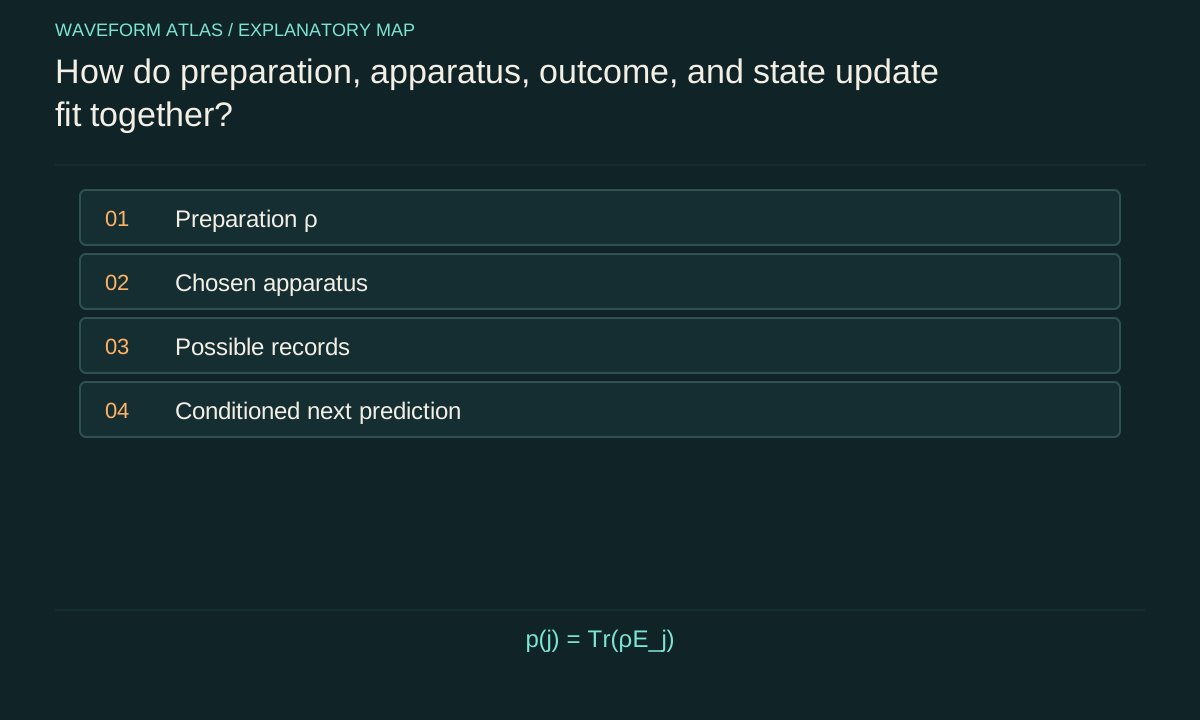
Begin with a question the apparatus can answer

A quantum measurement is a physical procedure that turns a question about a system into distinguishable records. The question might concern position, spin along a chosen axis, photon number or another observable. The apparatus does not simply expose an unlimited list of prewritten properties. Its coupling and readout determine which outcome probabilities are accessible and how the system is affected. Describing the apparatus is therefore part of describing the measurement.

A useful protocol has three stages: prepare a state, perform an interaction and record an outcome. Repeating the protocol produces a distribution of records. Quantum theory connects that distribution to the state and measurement description. One individual result does not reveal the entire state, and a detector label does not by itself identify an observable. Calibration establishes how known inputs map to records, allowing later data to be interpreted as answers to a defined physical question.

Separate amplitudes from probabilities

For a two-state system, write |ψ⟩ = a|0⟩ + b|1⟩ with |a|² + |b|² = 1. An ideal measurement in the zero/one basis gives probabilities |a|² and |b|². The complex amplitudes a and b can interfere in other measurements; the probabilities are nonnegative numbers that add to one. Confusing these two objects leads to errors such as adding amplitudes when the alternatives are distinguishable or discarding phase information when it matters.

Take a = √3/2 and b = 1/2. The zero/one probabilities are three quarters and one quarter. Changing the sign of b leaves those two probabilities unchanged, but it changes predictions in another basis. Thus a single set of outcome frequencies is generally insufficient to determine the state. Measurement is selective: it probes particular features through the apparatus chosen, rather than revealing every aspect of a quantum description at once.

The basis is a physical choice

Define |+⟩ = (|0⟩ + |1⟩)/√2 and |−⟩ = (|0⟩ − |1⟩)/√2. Measuring in this basis asks a different question from measuring zero versus one. For the state above, the plus probability is (1 + √3/2)/2, approximately 0.933. If the second amplitude has the opposite sign, that probability becomes approximately 0.067. The change is observable even though the zero/one statistics remain identical.

In a laboratory, a basis change can require rotating a spin, changing an optical analyzer or applying a controlled unitary before detection. It is not merely relabeling a graph. The same detector hardware can implement different measurements when preceded by different calibrated operations. Reporting the basis therefore means reporting the physical sequence and its reference axes or phases. Without that information, a probability table may be mathematically correct but experimentally ambiguous.

A record requires distinguishability

An ideal measurement interaction correlates system states with apparatus states: |0⟩|Aready⟩ becomes |0⟩|A0⟩ and |1⟩|Aready⟩ becomes |1⟩|A1⟩. If A0 and A1 are reliably distinguishable, the apparatus can identify the alternatives. If their probability distributions overlap, some records are ambiguous. Finite resolution, noise and missed events belong in the measurement model rather than being treated as an afterthought.

The coupling also explains backaction. A coherent input can become entangled with the apparatus, changing the statistics available from the system alone. This does not require a human to read the display. The physical record can exist in a photodetector, memory element or scattered field. Whether that process is described through state conditioning, global unitary evolution or additional dynamics is a further question; the operational probabilities and record quality still need to be specified.

General measurements go beyond projectors

An ideal projective measurement uses orthogonal projectors onto distinct subspaces. More general measurements are described by positive operators E_j that sum to the identity. Their probabilities are p(j) = Tr(ρE_j), where ρ is the density operator. These effects can represent inefficient detection, ambiguous outcomes and procedures implemented by coupling to an auxiliary system. They are not necessarily mutually orthogonal projectors.

The effects determine probabilities, but they do not uniquely determine the state after the measurement. A measurement instrument, often represented through operators M_jα, supplies that additional information. Its effects satisfy E_j = Σα M_jα†M_jα. Different instruments can share the same E_j while disturbing the system differently. This distinction becomes essential when predicting a second measurement, designing feedback or judging whether a readout preserves the property it is intended to measure.

Condition on a result without losing the ensemble

If an outcome j is known, the state assignment is updated using the corresponding instrument and normalized by p(j). If the result is ignored, the output is the sum over all possible outcomes. These are different predictions for different information conditions. The unconditioned state can be mixed even when each conditioned state is pure. A report should say whether its plots describe all trials or a selected subset with a known record.

For an ideal zero/one measurement of |+⟩, the conditioned output is |0⟩ or |1⟩. Ignoring the result gives an equal mixture. Measuring zero/one again immediately gives the same result within each ideal conditioned sequence. Measuring plus/minus instead gives equal probabilities. The order and the retained record both matter. These simple examples show why “the state after measurement” is incomplete unless the protocol and conditioning are stated.

Calibration connects equations to detector counts

Real detectors can miss events, confuse labels or produce background clicks. Suppose a detector identifies a true zero as zero with probability 0.98 and a true one as one with probability 0.95. An input distribution of 75% zero and 25% one then produces a reported-zero probability of 0.75×0.98 + 0.25×0.05 = 0.7475. The observed distribution is close to, but not identical with, the ideal Born-rule distribution.

This teaching calculation treats the errors as stable classical misclassification after an ideal measurement. Other devices require a genuinely different quantum measurement model. In either case, calibration uncertainty must propagate into the inferred state or parameter. Simply renaming every click as a perfect outcome can create false purity, spurious correlations or an apparent violation of a theoretical prediction. The response model is part of the evidence, not a cosmetic correction applied after the conclusion is chosen.

Measurement can be weak, repeated or destructive

A weak interaction acquires limited information per trial and can leave substantial coherence. A strong readout can sharply distinguish alternatives. A destructive detector may absorb the system, making a later measurement on that same particle impossible. A repeated nondemolition-style protocol aims to preserve a measured property under stated conditions. These categories describe different physical procedures, not different levels of an observer’s attention.

Repeated interrogation can alter later dynamics, as illustrated by quantum Zeno experiments on driven transitions. Weak measurement with postselection can yield unusual conditioned averages, but those averages must be interpreted with the full protocol. Neither phenomenon licenses the claim that measurement has no physical mechanism or can send information backward in time. The interaction, records, selection and resource costs remain central to understanding what the experiment establishes.

Keep operational success separate from foundational claims

Decoherence explains how coupling to an environment can suppress local interference and stabilize particular records. Objective-collapse proposals add new dynamics intended to select outcomes physically. Interpretations of standard quantum mechanics may explain the relation between the global state and records in other ways while preserving the same observable statistics. A successful detector does not by itself discriminate between all these accounts.

To test a modified dynamics, identify a prediction beyond ordinary measurement theory, such as additional heating, radiation or coherence loss with a specified scaling. To characterize a detector, use calibration and repeated statistics. To discuss the measurement problem, make clear which conceptual question remains after those operational tasks are solved. Separating these goals lets a reader appreciate both the practical precision of quantum measurements and the continuing foundational debate without treating one as evidence that the other has disappeared.

End with the next prediction

A measurement description is most useful when it predicts what happens next. State the preparation, basis, effects, instrument, retained records and detector response, then calculate a later observable. If two proposed descriptions give different later statistics, an additional experiment may distinguish them. If they agree for every accessible measurement in the protocol, the present data do not choose between them.

This viewpoint makes measurement a concrete chain of physical and statistical operations. It avoids picturing a detector as a passive window into every property or as a mysterious event outside physics. The apparatus asks a particular question, produces imperfect but calibratable records and changes the conditions for subsequent predictions. Understanding those three roles is the foundation for the more specialized pages on Born probabilities, weak measurement, repeated interrogation and the relation between decoherence and definite outcomes.

For example, a device that estimates a population accurately may still be unsuitable for preserving a superposition for a later gate. Its first-outcome statistics answer one question; its disturbance answers another. Choosing between devices therefore requires the intended sequence, not a single accuracy score. This is why a measurement specification should follow the whole experiment rather than end at the first click.

Go to the original work.

These links identify the sources behind specific claims. Verification scope varies by source and is stated below.

1. 1 / University teachingPreskill, Quantum Information, Chapter 3: Measurement and Evolution ↗

   Measurement operators, channels, dephasing, amplitude damping and open-system evolution.

   Verification scope: Author-hosted lecture PDF inspected for relevant sections; not an exhaustive audit of every lecture derivation.

2. 2 / University teachingPreskill, Quantum Information, Chapter 2: States and Ensembles ↗

   Density operators, composite states, measurement probabilities, quantum erasure and local statistics.

   Verification scope: Author-hosted lecture PDF inspected for relevant foundational definitions; independent elementary examples are worked in the article.

3. 3 / Primary theoryDressel et al., Understanding Quantum Weak Values: Basics and Applications ↗

   Weak measurement, conditioned averages and application-specific interpretation.

   Verification scope: Author-posted review abstract and publisher bibliographic record inspected.

4. 4 / Primary experimentItano et al. (1990), Quantum Zeno effect ↗

   Repeated physical interrogation inhibited a driven transition in trapped ions.

   Verification scope: NIST-hosted paper abstract and introductory derivation inspected; distinguish induced-transition protocol from every spontaneous decay.

5. 5 / Primary theoryZurek, Decoherence, einselection, and the quantum origins of the classical ↗

   Environmental monitoring, preferred records and suppression of local interference.

   Verification scope: Author-posted review abstract and bibliographic record inspected.

6. 6 / Primary theoryBassi et al., Models of Wave-function Collapse, Underlying Theories, and Experimental Tests ↗

   Research authors’ synthesis of stochastic collapse dynamics, motivation and distinct experimental signatures.

   Verification scope: Author-posted review abstract and bibliographic record inspected; general equations below are explicitly specified teaching models.