Losing a pattern without losing all its energy

A pattern is a relationship

Two beams can each maintain steady power while their interference pattern becomes unstable. The relevant quantity is not the power of either beam alone but the relative phase of their contributions at the detector. A stable phase produces a reproducible cross term. A phase that wanders over the measurement interval can make positive and negative contributions cancel in the average, leaving an apparently featureless sum of intensities.

The word scrambling is therefore incomplete without a reference. One must say which phases vary, relative to what, over which locations or trials, and with what information retained. A rough optical surface may impose a complicated but stable spatial phase pattern. A fluctuating frequency may produce a changing temporal phase. A quantum environment may carry information about alternative paths. These examples can all affect interference, but they are not one physical process.

The complex average contains the visibility

For two contributions with intensities I₁ and I₂, let their relative phase be φ₀+δφ. Averaging the intensity gives Ī=I₁+I₂+2√(I₁I₂)Re[exp(iφ₀)⟨exp(iδφ)⟩], under stable-amplitude and matching-mode assumptions. Define C=⟨exp(iδφ)⟩. Its magnitude controls the reduction in contrast and its argument shifts the fringe. This compact expression separates a mean phase displacement from a spread in phase.

For equal beam powers and otherwise perfect overlap, the fringe visibility is |C|. If δφ is equally likely to be any angle over a full cycle, C=0 and the averaged fringe disappears. Yet each individual realization may still contain a fully contrasted pattern at a different position. The average answers a question about the specified ensemble; it does not automatically describe what happened in every member of that ensemble.

A Gaussian example makes the scale concrete

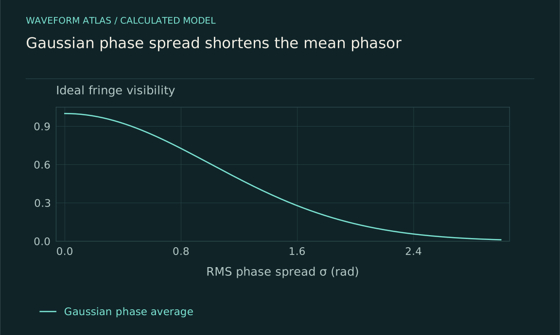
Assume the random phase has mean zero and a Gaussian distribution with variance σ², measured in radians squared. Its characteristic function gives C=exp(−σ²/2). An rms phase spread of 0.2 radians therefore leaves visibility about 0.980, while a spread of one radian leaves about 0.607. These are calculated values for a chosen statistical model, not universal thresholds for coherence.

A broad distribution need not be Gaussian. Two equally likely phases separated by π already give C=0, even though only two distinct settings occur. Conversely, a phase distribution with several narrow peaks can retain a nonzero complex average. Measuring one visibility number therefore does not reconstruct the distribution. Different noise statistics can produce the same first-order coherence while differing in time correlations or in their response to a pulse sequence.

A simple two-setting distribution provides another useful calibration. Let the phase be zero with probability p and π with probability 1−p. Then C=p−(1−p)=2p−1. At p=0.75 the visibility is 0.5, while at p=0.5 it vanishes. If p falls below one half, the fringe returns with a π shift because C becomes negative. Thus a decreasing population of one phase class can first erase and then restore contrast; monotonic language about increasing disorder would miss the sign change.

This example also separates visibility from information available in a record. If each trial is labeled with its selected setting, the two subsets can each show full contrast even when their unsorted average is flat. If labels are unavailable, that recovery is inaccessible through the local intensity data alone. The same photons or waves have not acquired extra energy when sorting restores the pattern; the analysis has recovered a relationship hidden by mixing different settings.

Keep energy and populations separate

Multiplying a field by exp(iφ) changes its complex phase but not its magnitude. In an ideal phase-only transformation, the intensity in that mode is unchanged at that instant. Subsequent propagation or recombination can redistribute intensity because the transformed field interferes differently with other contributions. A detector that sees less power in one output may therefore be observing a redistribution rather than absorption.

For a two-level quantum system, pure dephasing in the energy basis changes off-diagonal density-matrix elements while leaving the diagonal populations fixed. This is a statement about a specified model and basis. Real devices can combine dephasing with energy relaxation, leakage, heating, or technical loss. Measuring unchanged total counts or energy helps constrain those possibilities, but a complete claim requires the corresponding observables rather than the visual appearance of a fading fringe.

Known complexity is not necessarily lost control

Imagine a spatial phase mask that applies phases 0, π/2, π, and 3π/2 to four equal aperture segments. The far-field pattern can become complicated, but the transformation is known. Applying the opposite phases in the same plane restores the original field in the ideal model. Calling the intermediate wavefront disordered does not make its evolution irreversible.

The same distinction appears in time. A programmed phase modulation can produce a broad spectrum while remaining exactly synchronized to a reference. If the phase record is retained, a suitable analysis can undo the modulation or sort measurements by phase. If the record is discarded, the averaged description may look dephased. Whether information is unavailable in practice or destroyed by a proposed physical law is a separate question that the word random should not conceal.

Environments can carry the missing relation

Consider a joint state (|0>|E₀>+|1>|E₁>)/√2. The path coherence visible locally is proportional to ⟨E₁|E₀⟩. When the environment states become distinguishable, their overlap decreases and path interference weakens. The whole system can still evolve according to a reversible unitary model, even though an observer restricted to the paths cannot recover the phase through operations on those paths alone.

This mechanism differs from simply choosing an unknown classical phase on each trial, although the two can produce identical reduced density matrices. Joint measurements or retained preparation records may distinguish them. Local visibility alone cannot. The density-matrix description is useful precisely because it predicts accessible observations without pretending that the same local state determines a unique global history or interpretation.

Time scales determine what averaging hides

A slow phase drift may leave a short exposure sharply fringed while moving the fringes between exposures. A long exposure averages those positions and lowers contrast. Faster fluctuations can reduce contrast even within the shortest available exposure. Thus a reported coherence measurement depends on acquisition timing, reference stability, and detector bandwidth as well as on the underlying system.

Sampling can also miss fluctuations. A phase that changes between measurements may appear as independent noise, while a periodically sampled modulation can be mistaken for a stationary offset. Recording time stamps and a reference signal allows correlation analysis and checks for aliasing. The useful question is not merely whether phase varies, but which part of that variation the measurement resolves and which part it folds into an average.

Recovery tests identify some causes

A spin echo illustrates recovery of a phase spread produced by sufficiently stable frequency offsets. A refocusing pulse reverses the relative accumulation so that the ensemble can rephase later. Hahn's original work establishes the echo phenomenon; later pulse-sequence theory analyzes how control filters different noise processes. Neither result implies that arbitrary environmental interactions or all energy relaxation can be undone by a single pulse.

Other recovery tests include shortening an optical path imbalance, stabilizing a reference, sorting trials by recorded phase, or applying an inverse wavefront mask. Successful recovery supports a particular reversible or controllable mechanism. Failed recovery is less specific: the control may be imperfect, the environment inaccessible, or the assumed model wrong. The asymmetry between these inferences is important when interpreting a missing pattern.

A practical diagnostic sequence

Begin with independent intensity or population measurements. Then scan a controlled phase to determine contrast, mean phase, and their variation with delay. Repeat with different exposure times and monitor the reference. A loss of contrast accompanied by falling total counts suggests that attenuation or detection changes need attention; a phase-only explanation should not be assumed before those effects are checked.

Next perturb one suspected cause. Change the path delay, temperature stability, pulse sequence, or environment coupling while holding other parameters as steady as possible. Compare the resulting functional dependence with a stated model. A single fitted decay time summarizes data, but several mechanisms can share the same apparent decay over a limited interval. Multiple controls turn a descriptive curve into stronger evidence about the underlying process.

What the disappearing pattern establishes

A washed-out interference pattern establishes reduced coherence for the specified observable, averaging procedure, and reference. It does not alone establish zero energy, the absence of a wave in every realization, or a universal collapse mechanism. Those stronger conclusions require additional measurements and explicit theoretical predictions. The distinction keeps phase-sensitive experiments useful without asking them to answer questions they were not designed to resolve.

The productive way to read phase scrambling is as a family of mechanisms that alter accessible relationships. Determine whether the phase is known, statistically distributed, dynamically fluctuating, or stored in correlations with another system. Then choose a measurement that distinguishes those alternatives. That sequence explains both why an interference pattern can disappear and why, in some carefully controlled settings, it can return.

Go to the original work.

These links identify the sources behind specific claims. Verification scope varies by source and is stated below.

1. 1 / University teachingMIT: Demonstrations in physical optics ↗

   MIT: Demonstrations in physical optics. https://ocw.mit.edu/courses/res-6-006-video-demonstrations-in-lasers-and-optics-spring-2008/pages/demonstrations-in-physical-optics/

   Demonstrations identify amplitude, polarization, vibration, path difference and spectrum as controls on fringe contrast.

   Verification scope: Official course demonstration index and descriptions inspected.

2. 2 / University teachingMIT: Entanglement, Density Matrices, and Decoherence ↗

   Aram W. Harrow (2016). 8.06 Chapter 3: Entanglement, Density Matrices, and Decoherence. MIT OpenCourseWare.

   Density operators and reduced states distinguish local observables from joint correlations.

   Verification scope: Official full chapter text inspected at §§1–4 for states, density operators and reduced dynamics, and §5.1 for interference and environmental records. Worked examples in this article are independent calculations.

3. 3 / Primary experimentSpin Echoes ↗

   E. L. Hahn. Physical Review 80, 580–594 (1950).

   DOI: 10.1103/PhysRev.80.580

   Pulse sequences can refocus an ensemble of spins and reveal relaxation.

   Verification scope: Publisher or author-institution abstract and bibliographic record inspected; full paper not audited.

4. 4 / Primary theoryHow to enhance dephasing time in superconducting qubits ↗

   Łukasz Cywiński; Roman M. Lutchyn; Cody P. Nave; S. Das Sarma. Physical Review B 77, 174509 (2008).

   DOI: 10.1103/PhysRevB.77.174509

   Pulse sequences filter specified noise and can support noise spectroscopy.

   Verification scope: Publisher or author-institution abstract and bibliographic record inspected; full paper not audited.