Recovering coherence lost to a known spread

A fading ensemble can contain coherent members

An ensemble of spins in a magnetic field can precess at slightly different rates because the field varies across the sample. Immediately after preparation, their transverse contributions may point in the same direction. Later they fan out in phase, and their vector sum becomes small. Each member can still have a well-defined transverse phase even though the summed signal has faded.

Hahn's 1950 work demonstrated spin echoes produced by radiofrequency pulse sequences and connected echo amplitudes to relaxation measurements. The central lesson is that some apparent decay reflects phase dispersion that can be refocused. It is not evidence that every lost signal is recoverable. The original abstract also recognizes diffusion as relevant to interpretation, emphasizing that an echo experiment probes dynamics as well as an ideal geometric reversal.

Work in a rotating reference frame

Choose a frame rotating at the reference angular frequency. A spin packet with offset Δ then accumulates relative phase Δt. If all packets begin along the same transverse direction, their phases after time τ are Δτ. Positive and negative offsets lie on opposite sides of the reference direction. The measured transverse signal is proportional to the vector sum over the distribution of offsets.

For a Gaussian distribution with rms width σΔ, ideal free induction has envelope exp(−σΔ²t²/2), ignoring other decay mechanisms. This is a calculated ensemble result, not a statement that each packet's own transverse magnitude has diminished. It provides a clear example of why a short apparent decay time can arise from static inhomogeneity rather than rapid irreversible relaxation.

The refocusing pulse changes phase ordering

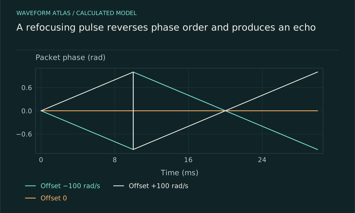
Apply an ideal π rotation about a transverse axis at time τ. With a suitable axis convention, a transverse phase φ is mapped to −φ. A packet that had accumulated Δτ therefore begins the second interval at −Δτ. It continues precessing with the same offset Δ, reaching phase −Δτ+Δτ=0 at time 2τ. All static offsets rephase at that moment.

The pulse does not generally make fast spins physically precess slowly. It reflects their phase positions so that continuing at their original rates brings them together again. This distinction makes the timing transparent and avoids an inaccurate picture of reversing every microscopic motion. The MIT laboratory handout describes this phase-refocusing geometry and the appearance of the echo after a second equal interval.

Three packets illustrate the arithmetic

Take offsets −100, 0, and +100 radians per second and let τ=10 milliseconds. Just before the π pulse, their phases are −1, 0, and +1 radians. Immediately after the ideal reflection, they are +1, 0, and −1. Another ten milliseconds of free evolution brings all three to zero relative phase. The ensemble signal is then restored in this ideal model.

At a time δt away from the echo center, the phases again spread as Δδt. The echo is therefore a peak with a width related to the offset distribution, not a permanent restoration of aligned phases. If no further control is applied, the ensemble dephases again. The experiment has arranged a specific rephasing time rather than removed the underlying inhomogeneous frequencies from the sample.

An error in the pulse timing also has a simple signature. Keep the intended readout at 2τ but apply the pulse at τ+ε. A static packet then accumulates −Δ(τ+ε)+Δ(τ−ε)=−2Δε by the readout. The echo center shifts to twice the actual pulse time, and reading at the old center produces residual phase spread. With a Gaussian offset width σΔ, the ideal signal at that mistimed readout is reduced by exp(−2σΔ²ε²).

This calculation separates a timing error from loss of transverse magnitude. Scanning the readout time can locate the shifted echo and recover its peak, whereas a true reduction of the envelope remains after that adjustment. For σΔ=100 radians per second and ε=1 millisecond, the predicted factor is about 0.980. The example supplies a concrete calibration test and shows why echo amplitude should be extracted from the measured peak position rather than from an assumed fixed sample time.

Changing offsets leave a residual phase

Suppose one packet experiences offset Δ₁ in the first interval and Δ₂ in the second. After refocusing, its net phase is (Δ₂−Δ₁)τ. A stable offset cancels, but a changed offset does not. If the two offsets differ by 20 radians per second and τ=10 milliseconds, the residual is 0.2 radians. A distribution of such changes reduces the ensemble echo.

Motion through a spatial field gradient can create precisely this problem: a spin samples different fields before and after the pulse. Random temporal noise can do the same without motion. The echo response therefore depends on correlations across the two intervals. A small echo cannot be assigned uniquely to one relaxation process unless these additional contributions are modeled or controlled.

Distinguish T₂, T₂* and T₁

T₁ conventionally describes recovery of longitudinal populations or magnetization in an appropriate relaxation model. T₂ describes transverse coherence decay after accounting for the specified refocusable inhomogeneity. T₂* commonly includes that inhomogeneous broadening in the observed free-induction decay. Their numerical relation depends on the assumed line shapes and dynamics; not every decay is a single exponential with a unique rate.

In a simple Markovian two-level model, 1/T₂=1/(2T₁)+1/Tφ, where Tφ characterizes additional pure dephasing. This model implies T₂≤2T₁. The relation should not be indiscriminately applied to an arbitrary multilevel ensemble, nonexponential decay, or fitted echo envelope. Define the observable and model before turning a measured time constant into a statement about microscopic energy exchange.

Pulse errors can imitate imperfect recovery

A real pulse has finite duration, nonuniform amplitude, and possible frequency detuning. Different spins may undergo rotations that differ from the intended π angle or axis. The resulting echo can be smaller even when the static offset distribution would otherwise be refocusable. Calibrating pulse area and phase is therefore part of measuring the sample, not merely a preliminary technical detail.

Receiver recovery after a strong pulse can also obscure early signals. If the electronics are temporarily saturated, a missing feature may be an instrument effect. Vary pulse amplitude, duration, and spacing while monitoring calibration signals. A decay that changes substantially with these settings needs a control-error model before being interpreted as an intrinsic coherence limit. More pulses can improve filtering while also accumulating more pulse errors.

Echo sequences are selective filters

For a single echo, the effective phase accumulation has opposite signs in the two halves. This cancels a constant offset and suppresses sufficiently slow variations. A longer pulse sequence creates a different temporal weighting and therefore a different response to the noise spectrum. The source by Cywiński and colleagues supports the connection between designed pulse sequences, coherence protection and noise inference in specified qubit models.

The filtering view explains why one sequence may outperform another in one environment but not in another. Pulse timing must match the noise being suppressed, and the approximation of instantaneous ideal pulses can fail. An echo is not a universal time-reversal operation. It reverses a controlled contribution to phase accumulation while leaving other Hamiltonian terms and dissipative channels potentially active.

Measure an envelope without hiding its assumptions

Acquire echoes at several total evolution times and retain the complete time trace around each echo. Extract amplitude using a consistent phase-sensitive or magnitude-based procedure, stating any background correction. Magnitude estimates near the noise floor can have a positive bias, so fitting a logarithm of raw magnitude may overestimate long-lived coherence. Include uncertainty and test whether the chosen decay law describes the data adequately.

Repeat with altered gradients, pulse calibration, or sample conditions when those changes can separate mechanisms. A comparison between free induction and echo directly demonstrates that some phase dispersion is refocusable. It does not by itself quantify every source of irreversible relaxation. The measured envelope is the response of a sample plus a control and detection protocol, and its interpretation should retain those ingredients.

A separate pulse-calibration run can measure the rotation angle as pulse duration varies. Repeating that calibration across the relevant frequency-offset range tests whether the nominal π pulse acts uniformly on the ensemble. The resulting bandwidth check helps distinguish imperfect refocusing from sample dynamics when the echo envelope changes.

What an echo proves about phase information

A recovered signal shows that the control sequence exploited phase relationships that were not visible in the earlier summed signal. It establishes a form of recoverability for the degrees of freedom and time scales tested. It does not show that all environmental records vanished, that energy relaxation was undone, or that a fundamental collapse process was reversed.

The strongest conclusion follows the explicit geometry: stable frequency differences produced a phase fan, a calibrated pulse reflected that fan, and subsequent evolution brought it together at the predicted time. Deviations then become useful data about noise, motion, relaxation and control. This turns the echo from a seemingly paradoxical return of a lost signal into a precise probe of which parts of an apparent decay were phase dispersion.

Go to the original work.

These links identify the sources behind specific claims. Verification scope varies by source and is stated below.

1. 1 / Primary experimentHahn (1950), Spin Echoes ↗

   Pulse sequences can refocus an ensemble of spins and reveal relaxation.

   Verification scope: Publisher abstract and bibliographic record inspected; no claim of full-paper review.

2. 2 / University teachingMIT Junior Lab: Pulsed Nuclear Magnetic Resonance: Spin Echoes ↗

   Echo timing, refocusing of static frequency spread, and limitations from relaxation and diffusion.

   Verification scope: Official university laboratory handout retrieved and relevant echo sections inspected.

3. 3 / Primary theoryCywiński et al. (2008), How to enhance dephasing time in superconducting qubits ↗

   Pulse sequences filter specified noise and can support noise spectroscopy.

   Verification scope: Publisher abstract and bibliographic record inspected; no claim of full-paper review.