What phase scrambling does not establish

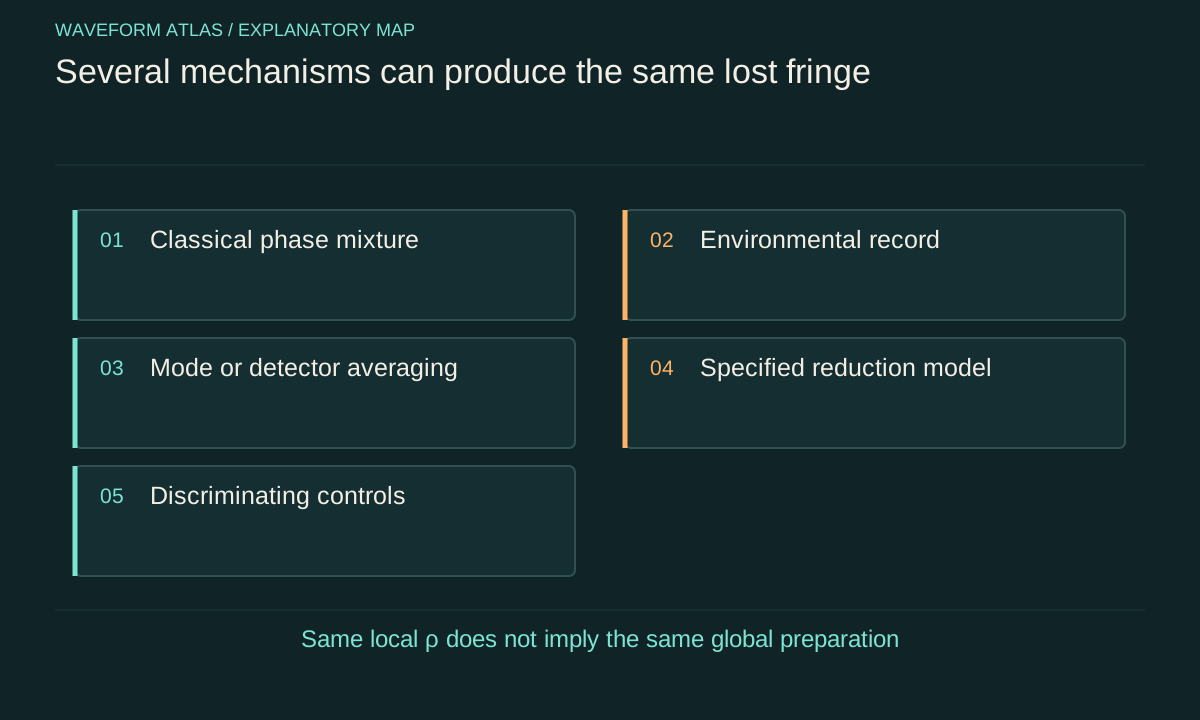
Begin with the observable, not its label

Suppose an interferometer's fringe visibility falls from nearly one to nearly zero. The measured fact concerns a phase-dependent modulation under a particular preparation, reference, detector geometry and averaging time. It does not directly state whether the field lost energy, whether each trial remained coherent, or whether the complete quantum state underwent a fundamental reduction. Those are possible interpretations requiring additional information.

Calling the result phase scrambling can be a useful descriptive shorthand, but it does not specify a law of motion. Calling it collapse adds an even stronger claim unless the term is explicitly being used for a conventional conditional state update after a measurement. A careful comparison therefore starts by writing candidate mechanisms and identifying what they predict for the actual recorded quantities.

Classical phase averaging is one candidate

Let each trial prepare (|0>+exp(iφ)|1>)/√2 with an unknown phase φ. If φ is uniformly distributed, the average path density matrix is I/2. A recombiner then shows no phase-dependent fringe in the pooled data. Every trial in this preparation can nevertheless be a pure coherent state. The loss of the averaged cross term comes from mixing different phases.

A retained phase record changes what can be inferred and recovered. Sorting or correcting trials by that record can reveal full conditional contrast. Without the record, local measurements are described by the mixture. This is an information and preparation issue within ordinary quantum statistics, not evidence that a new stochastic law selected one path on each trial. The same flat average is compatible with many different microscopic histories.

Environmental correlations are another candidate

A joint state (|0>|E₀>+|1>|E₁>)/√2 with orthogonal environment records also gives local path state I/2. Here the local mixedness comes from tracing over an entangled environment rather than from the particular classical preparation above. The joint state can remain pure. Path-only measurements cannot distinguish these two cases because their reduced density matrices are identical.

Access to the environment can reveal the difference through joint correlations or conditional measurements. In a controlled small system, reversing the interaction can restore the original path coherence. In a large environment, the necessary control may be unavailable. Practical irreversibility can be severe without the local fringe alone proving fundamental nonunitarity of the complete state. The system boundary is therefore central to the interpretation.

Ordinary apparatus effects can also flatten a fringe

Unequal arm powers, polarization mismatch, spatial misalignment, detector background and integration across moving fringes can all reduce observed visibility. Some change the interfering mode overlap; others change the measurement's weighting. A detector that averages over several spatial periods may record no modulation even though a resolved image would show sharp fringes. No dynamical collapse is needed to explain that effect.

Loss can additionally reduce count rates, and postselection can alter normalized statistics of the surviving sample. Measure individual inputs, total detected events and complementary outputs before assigning the residual behavior to dephasing. A good foundational experiment must handle these ordinary possibilities precisely because the desired signal often appears as a small deviation in the same quantities they affect.

A reduced channel does not identify a unique environment

Consider the dephasing map ρ↦(1−p)ρ+pZρZ, where Z changes the sign of one basis component. Its off-diagonal entries are multiplied by 1−2p while its populations remain unchanged. This map can be implemented by a classical random phase flip or by a suitable interaction with an unobserved ancillary system. Local process measurements can characterize the map without uniquely determining its physical implementation.

At p=1/2 the off-diagonal entries vanish. At p=1 the operation is a deterministic phase flip and coherence magnitude is fully preserved, with its phase reversed. This example shows why a parameter casually called noise strength must be interpreted within the actual model. The local channel is a predictive object; a statement about fundamental collapse is an additional claim about what physically realizes or modifies that channel.

A process can also look Markovian over one time range and reveal memory over another. For example, a classical static frequency offset produces a Gaussian free-evolution envelope, while an appropriate echo can cancel its accumulated phase. A memoryless exponential dephasing channel predicts a different response to the same idealized intervention. Observing only one decay curve loses that distinction; inserting controlled operations between preparation and readout tests the temporal structure of the process.

This is why even detailed local process characterization at a single time does not necessarily identify a unique dynamical mechanism. Measurements at multiple times and under interventions add information about correlations and memory. They still require assumptions about preparation and control accuracy, but they provide a more discriminating basis for theory comparison than assigning a fundamental meaning to a single fitted decay constant.

Conditional measurement is a separate operation

A projective measurement with recorded outcome j assigns the conditional state PⱼρPⱼ/Tr(Pⱼρ). If the outcome is ignored, the associated channel is ΣⱼPⱼρPⱼ. These formulas distinguish an outcome-conditioned description from an unconditioned ensemble. They should not be conflated with a phase shift or with a phase average performed before any detector record is considered.

Different interpretations of standard quantum theory can agree on these operational predictions while describing the status of the state differently. An objective-collapse theory generally proposes extra physical dynamics intended to address that status. Observing an ordinary detector outcome or applying the standard update rule does not by itself test the additional dynamics. A test requires a regime in which the proposed theory predicts something measurably different.

What a competing dynamical model must specify

A quantitative proposal needs the affected degrees of freedom, the basis or spatial structure of the reduction, its rate or parameters, and the resulting observable predictions. It must also say how ordinary environmental effects are included. Depending on the model, additional signatures might involve dependence on mass distribution, separation, time, diffusion or energy transfer. None of these dependencies follows merely from the word collapse.

The experiment should compare those predictions with a baseline model under the same preparation and measurement conditions. If both predict the same visibility curve within sensitivity, the result does not discriminate between them. If one predicts an additional effect, the analysis must identify the parameter range actually tested. Excluding one parameter choice is not equivalent to excluding every possible reduction model or resolving the measurement problem in general.

Recovery provides useful but limited evidence

A restored fringe after phase correction supports the claim that the tested loss was recoverable through that correction. A spin echo supports refocusing of particular phase accumulation. Conditional fringes support correlations with the sorting record. These are positive demonstrations of specific structure that a flat unconditioned signal hid. They can rule out explanations that would forbid the observed recovery under the tested assumptions.

Failure to recover is weaker evidence. The inverse may be inaccurate, the reference noisy, or the relevant environment inaccessible. A recovery protocol designed for static offsets will fail against sufficiently changing offsets even within ordinary dynamics. Therefore, an unsuccessful echo or compensation is not automatically evidence for fundamental collapse. The protocol's predicted response to known alternatives must be established first.

The amount recovered also needs a baseline. Compare the corrected signal with the contrast achievable at zero evolution time under the same readout, rather than with an ideal value the apparatus never attained. This separates a persistent preparation or detection limitation from the additional loss the recovery protocol was designed to address.

Build a discriminating measurement set

Measure visibility together with source power, populations or total counts, phase drift, and environmental controls appropriate to the setup. Vary a parameter for which candidate mechanisms predict different behavior. Change integration time to test averaging, reverse a known phase mask to test deterministic scrambling, or vary a tagging interaction to test environmental records. Use independent calibration data to constrain technical explanations.

When a new model predicts a distinctive dependence, preregistering or otherwise fixing the analysis choices before examining the relevant result can reduce selection bias. The key scientific requirement is transparent inference, not a particular administrative ritual. Report residuals, uncertainties and alternative fits so readers can see whether the proposed mechanism is required by the data or merely compatible with it.

State the conclusion at the level of the evidence

A justified conclusion might say that coherence decayed under a specified protocol, that an echo recovered a defined fraction, or that a parameterized extra-dephasing model is constrained within a measured range. These statements preserve the result's value while keeping its logical scope clear. A universal assertion that phase scrambling proves objective collapse exceeds what an unqualified visibility measurement can establish.

The distinction is productive rather than merely cautious. It tells an experimenter which next measurement would matter: a phase record, an energy monitor, a joint correlation, a recovery operation, or a parameter sweep. By separating observable loss of interference from the proposed mechanism, one can design tests that genuinely distinguish explanations instead of relabeling the same flat pattern several different ways.

Go to the original work.

These links identify the sources behind specific claims. Verification scope varies by source and is stated below.

1. 1 / University teachingMIT: Entanglement, Density Matrices, and Decoherence ↗

   Aram W. Harrow (2016). 8.06 Chapter 3: Entanglement, Density Matrices, and Decoherence. MIT OpenCourseWare.

   Density operators and reduced states distinguish local observables from joint correlations.

   Verification scope: Official full chapter text inspected at §§1–4 for states, density operators and reduced dynamics, and §5.1 for interference and environmental records. Worked examples in this article are independent calculations.

2. 2 / ReviewModels of wave-function collapse, underlying theories, and experimental tests ↗

   A. Bassi, K. Lochan, S. Satin, T. P. Singh, and H. Ulbricht. Reviews of Modern Physics 85(2), 471–527 (2013). Linked record is the author preprint.

   DOI: 10.1103/RevModPhys.85.471

   Collapse-model framework, stochastic modifications of quantum dynamics and model-specific experimental tests.

   Verification scope: Publisher or author-institution abstract and bibliographic record inspected; full paper not audited.