Probabilities from quantum amplitudes

Start with normalization

A quantum state vector represents probability amplitudes, not a list of probabilities. For |ψ⟩ = a|0⟩ + b|1⟩ in an orthonormal basis, normalization requires |a|² + |b|² = 1. The Born rule assigns probabilities |a|² and |b|² to an ideal measurement in that basis. In this basis, |a|² and |b|² are independent of both the overall phase and the relative phase. The relative phase remains in the state amplitudes and can affect probabilities after a change of measurement basis.

The normalization condition is not optional bookkeeping. If someone writes amplitudes 0.8 and 0.6, their squares add to one and the state is normalized. If they write probabilities 0.8 and 0.6, the proposed exhaustive outcomes sum to 1.4 and cannot be a valid probability distribution. The same numbers can play different roles in different expressions. Explicitly naming the role prevents a basic arithmetic mistake from becoming a supposed paradox about quantum uncertainty.

Calculate a simple distribution

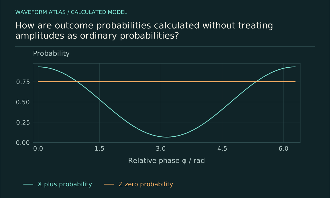
Consider |ψ⟩ = √(3/4)|0⟩ + e^{iφ}√(1/4)|1⟩. Measuring zero versus one gives p(0) = 0.75 and p(1) = 0.25 for every φ. In an ideal sequence of independently prepared trials, the expected number of zero results in N trials is 0.75N. That expectation is not a promise that every block of four trials contains exactly three zeros. Individual sequences fluctuate.

For N = 400, the binomial standard deviation of the zero count is √[400×0.75×0.25], about 8.66. The standard deviation of the observed fraction is about 0.0217. A count different from 300 is therefore normal, not a failure of the probability rule. This calculation assumes independent trials with the same state and stable apparatus. Drift, memory or changing preparation can invalidate the simple binomial model and should be checked rather than absorbed into a vague statement that quantum outcomes are random.

The count calculation is derived here: for independent indicators X_i equal to one on a zero outcome, E[X_i] = p and Var(X_i) = p(1−p). Adding N independent indicators gives count variance Np(1−p), and dividing by N² gives the fraction variance p(1−p)/N. Preskill is cited for the state probabilities, not this sampling derivation.

Reveal the relative phase with another basis

Use |+⟩ = (|0⟩ + |1⟩)/√2. The amplitude for a plus result is ⟨+|ψ⟩, so its probability is one half times the squared magnitude of √3/2 + e^{iφ}/2. Expanding gives p(+) = [1 + (√3/2)cos φ]/2. At φ = 0 this is about 0.933; at φ = π/2 it is 0.5; at φ = π it is about 0.067.

The zero/one probabilities are unchanged across these examples, but the plus/minus probabilities are not. This is why phase cannot be discarded merely because a particular measurement does not reveal it. A state is more than one probability histogram. The basis-dependent amplitudes encode interference possibilities across different measurement choices, and a complete characterization requires enough independent observables to distinguish those possibilities.

Add amplitudes only for indistinguishable alternatives

When two coherent alternatives lead to the same unresolved outcome, their amplitudes add before the magnitude is squared. If their amplitudes are a and b, the probability contains |a+b|², including the interference term 2Re(a*b). If an accessible record distinguishes the alternatives and that record is ignored, the relevant local probability can instead become |a|² + |b|². The difference is physical: information about the alternatives has changed the joint state or the measurement.

This rule does not mean that an observer’s ignorance magically creates interference. Alternatives can be distinguishable through an unobserved environment even when nobody knows the record. Conversely, erasing a label on a notebook does not undo a physical which-path correlation. The calculation must describe the actual state and the degrees of freedom included in the measurement. Only then can one decide whether amplitudes or probabilities are being combined.

Use density operators for mixtures and subsystems

A density operator ρ describes both pure states and statistical mixtures. For a pure state, ρ = |ψ⟩⟨ψ|. For a mixture, ρ = Σk qk|ψk⟩⟨ψk| with nonnegative weights summing to one. The Born rule for an outcome represented by a projector P_j is p(j) = Tr(ρP_j). The trace formula reproduces the squared-amplitude rule and also handles states that cannot be represented by one vector.

Different ensemble decompositions can yield the same ρ and therefore the same local measurement statistics. This is important when a subsystem is entangled with something else. Its reduced density operator may be mixed even though the joint state is pure. The local probabilities are calculated from the reduced state; they do not reveal which ensemble story was used to write that matrix. Additional correlations must be measured to distinguish global preparations.

Generalize the outcome description

For a general measurement, replace projectors with positive effects E_j that sum to the identity. The probability remains p(j) = Tr(ρE_j). Positivity ensures nonnegative probabilities, and completeness ensures that all listed outcomes sum to one. An inefficient detector can include an explicit no-click effect rather than pretending every trial produces a successful event. Ambiguous outcomes can be included as outcomes rather than silently discarded.

This mathematical generalization is useful because real measurement procedures can couple the system to an auxiliary device, read only part of that device and coarse-grain several underlying events into one label. The effects summarize the resulting probabilities. They do not yet determine the post-measurement state; that requires an instrument. The Born rule answers how often records occur, while the instrument answers how the system is transformed in association with those records.

Keep conditional probabilities normalized

Postselection means retaining only trials with a specified event. If A and B are recorded events, the conditional probability p(A|B) is p(A and B)/p(B), provided p(B) is nonzero. The denominator matters. A striking pattern in a rare selected subset can coexist with an unremarkable distribution over all trials. Reporting the selected pattern without its success probability can exaggerate the information or sensitivity gained by the procedure.

For a simple example, suppose 10% of trials meet a selection criterion and 90% of those selected trials have property A. The joint fraction is 9% of all trials, not 90%. In quantum protocols, amplitudes and measurement backaction determine the relevant joint probabilities, but the final conditioning still follows probability theory. Postselection does not permit a local observer to access a remote selection record without communication, and it does not override normalization.

Separate preparation errors from probability-law tests

If observed frequencies disagree with an ideal prediction, several explanations should be checked before proposing a failure of the Born rule. The prepared state may differ from the intended state, the basis rotation may be miscalibrated, the detector may confuse outcomes or the trials may not be independent. A test of the probability law requires controls that distinguish these possibilities from the proposed deviation.

Suppose the intended plus state is actually dephased, with off-diagonal elements reduced by a factor c. A plus-basis measurement then gives p(+) = (1+c)/2 instead of one. This is a conventional change in the state, fully compatible with the Born rule. Calling the lower success probability a failure of the rule would conflate the state preparation with the mapping from a state to probabilities. The model being tested must include both pieces separately.

Understand what a frequency estimate establishes

For interpreting finite data, this atlas uses the following statistical cautions. Repeated counts estimate probabilities under a stable protocol. They do not prove that a finite dataset contains the exact theoretical distribution. Confidence intervals or other uncertainty summaries quantify how much variation is expected under the analysis assumptions. Small samples can easily miss rare outcomes, and a zero observed count does not establish a zero underlying probability. The interpretation should match the sample size and the statistical method used.

A frequency estimate also does not automatically establish purity. The state |+⟩ and a fifty-fifty mixture of |0⟩ and |1⟩ give identical zero/one counts. Measuring another basis separates them. This illustrates a broader principle: no amount of precision in one incomplete measurement substitutes for the missing observables needed to identify a state. Better statistics and a more informative protocol solve different problems.

The lecture reference supports the final comparison of states and measurement bases; the finite-sample cautions above are methodological advice.

Use the rule without overselling its foundations

The Born rule is a central operational rule of quantum theory, and the calculations above show how it is used. Different foundational programs debate how it should be understood or derived from a broader account. Those debates should not be confused with the practical task of applying the rule to a specified preparation and measurement. Conversely, using the rule successfully does not select a unique interpretation of the quantum state.

A clear calculation ends with a normalized distribution, a statement of the measurement effects and an explanation of which phases or correlations the apparatus can access. A clear experiment adds calibration, repeated-trial assumptions and uncertainty. Together these steps make the connection between amplitudes and data precise. They also reveal where a surprising result should lead next: to improved preparation checks, a different basis, a refined detector model or, only with sufficiently discriminating evidence, a test of new physical dynamics.

A final arithmetic check is to sum all mutually exclusive outcomes before interpreting a selected subset. If the total differs from one, identify whether an outcome was omitted, a probability density was mistaken for a probability or the state was left unnormalized. This elementary check often resolves an apparent anomaly before any foundational explanation is needed.

Go to the original work.

These links identify the sources behind specific claims. Verification scope varies by source and is stated below.

1. 1 / University teachingPreskill, Quantum Information, Chapter 2: States and Ensembles ↗

   Preskill, J. Quantum Information, Chapter 2: States and Ensembles. Caltech lecture notes (2015 version).

   Pure states, density operators, partial trace, pure-state entanglement, Born probabilities and quantum erasure. Does not supply mixed-state witnesses, entropy or quadrature formulas cited elsewhere.

   Verification scope: Author-hosted lecture PDF inspected for relevant foundational definitions; independent elementary examples are worked in the article.

2. 2 / University teachingPreskill, Quantum Information, Chapter 3: Measurement and Evolution ↗

   J. Preskill (2018). Lecture Notes for Ph219/CS219, Chapter 3: Foundations II: Measurement and Evolution, updated October 2018. Caltech.

   Quantum measurement operators and instruments, channels, dephasing, amplitude damping and open-system evolution. Not a detector-calibration or sampling-statistics handbook.

   Verification scope: Author-hosted lecture PDF inspected for relevant sections; not an exhaustive audit of every lecture derivation.

3. 3 / Primary theoryModels of wave-function collapse, underlying theories, and experimental tests ↗

   A. Bassi, K. Lochan, S. Satin, T. P. Singh, and H. Ulbricht. Reviews of Modern Physics 85(2), 471–527 (2013). Linked record is the author preprint.

   DOI: 10.1103/RevModPhys.85.471

   Research authors’ synthesis of stochastic collapse dynamics, motivation and distinct experimental signatures.

   Verification scope: Author-posted abstract and APS journal record inspected. Supports collapse-model motivation, dynamical modifications and experimental signatures; not the article’s independent calculations or reporting advice.