Reflection at an impedance boundary
Adjust the controls, inspect the calculated response and use the reading links to place the model in its physical context.
Interactive model: Reflection at an impedance boundary. Enable JavaScript to adjust its controls.
R = [(Z₂ − Z₁)/(Z₂ + Z₁)]²; T = 1 − R
Lossless acoustic plane waves at normal incidence between two positive real impedances. The coefficients are energy fractions; pressure-amplitude transmission can exceed one without creating energy.
What this model assumes
Lossless acoustic plane waves at normal incidence between two positive real impedances. The coefficients are energy fractions; pressure-amplitude transmission can exceed one without creating energy.
How to explore it
Begin with the default values. Change one control at a time and watch both the graph and the readouts. Then reset the model and change another parameter. This isolates which input produces the effect you are seeing.
The plotted values are generated from the displayed equation. Downloading the calculated data lets you inspect the numerical series or compare it with a calculation of your own. The data are synthetic model outputs, not observations from an apparatus.
Before carrying a prediction into an experiment, match the model’s assumptions to the actual system: the relevant degrees of freedom, boundary conditions, noise, losses and measurement convention. The linked articles explain which comparison is physically meaningful.
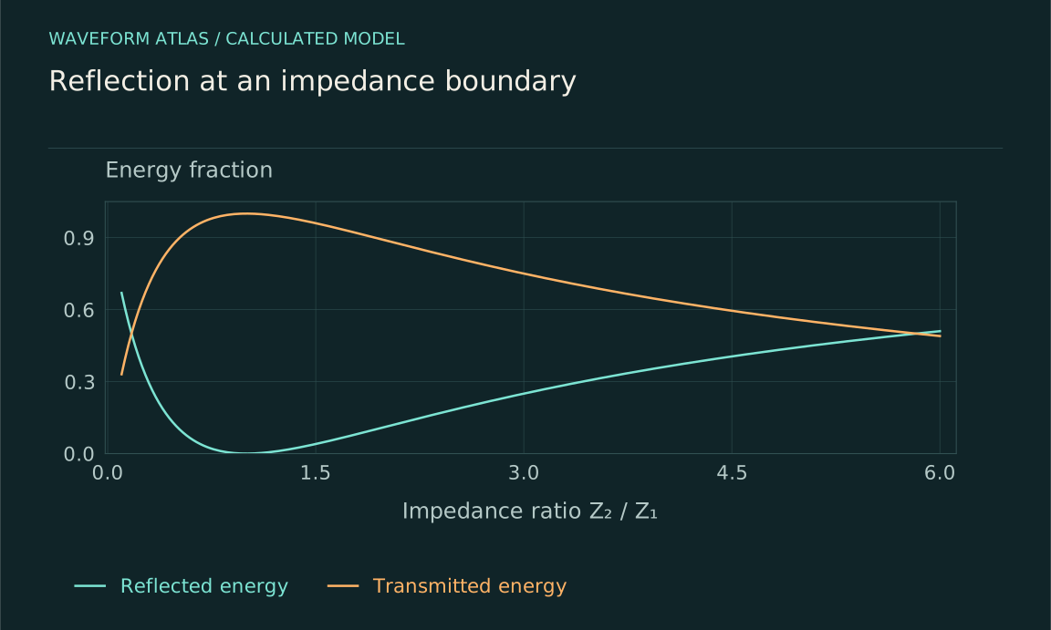
Calculated model curves. Lossless acoustic plane waves at normal incidence between two positive real impedances. The coefficients are energy fractions; pressure-amplitude transmission can exceed one without creating energy. Default control values are used in this fixed figure.
Download SVG ↓Changing the medium
Change the medium, change the propagation
Which properties of a carrier or material govern a particular wave?
Why waves reflect at mismatched media
What does wave impedance measure and why does a boundary matter?
More than a change in direction
How do refractive response, wavelength, and phase velocity relate?
Different frequencies, different propagation
How does a medium reshape a pulse without necessarily absorbing it?
Direction-dependent wave behavior
What changes when a material responds differently along different axes?
A medium that changes from place to place
How can a gradual gradient bend or focus a wave?
A material that changes while the wave is inside it
How can temporal modulation exchange energy with a field?
When the medium’s response depends on the wave
What new behavior appears beyond a linear constitutive law?
Measure the medium before explaining the wave
Which measurements identify the material parameters a model needs?
Choosing a medium for a desired wave transformation
How do loss, bandwidth, fabrication, and stability constrain a design?