When the medium’s response depends on the wave

Linear response has a testable meaning

A system is linear when its response to a sum of inputs equals the sum of its responses to those inputs, and scaling an input scales the output by the same factor. This superposition property allows frequency components to propagate independently in a time-independent medium. A nonlinear constitutive law breaks that property because the induced response contains products or other nonlinear functions of the field.

Nonlinearity is not synonymous with a complicated waveform. A linear dispersive system can reshape a pulse dramatically while still obeying superposition. Conversely, a weak nonlinear correction can matter after a long propagation distance even when the output initially looks almost sinusoidal. Test amplitude scaling and combined-input behavior rather than classify the mechanism from visual complexity alone.

A polynomial response shows new frequencies

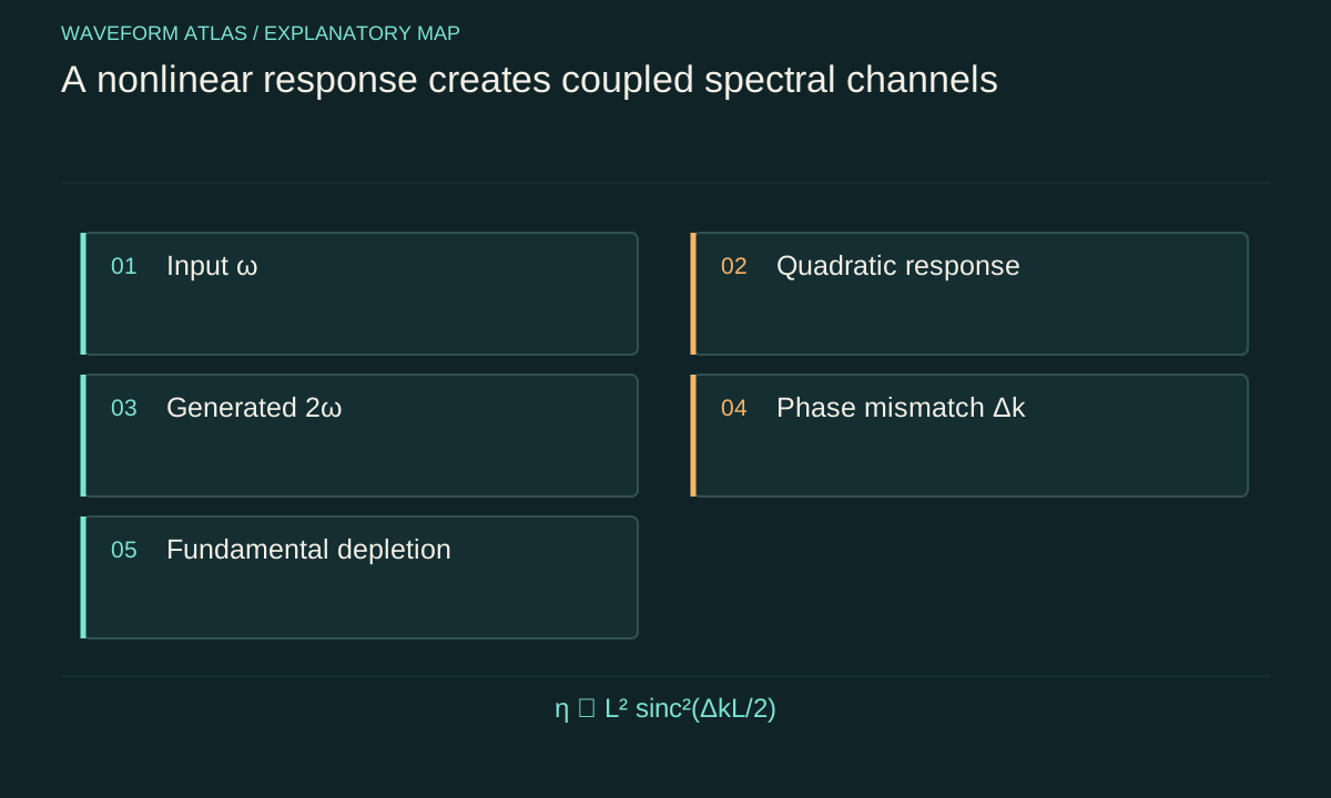
In a simplified scalar optical model, polarization can be expanded as P = ε₀(χ₁E + χ₂E² + χ₃E³ + …). The coefficients and allowed tensor components depend on the material and geometry. If E = E₀ cos ωt, the square contains a constant term and a component at 2ω. The cube contains components at ω and 3ω. The material can therefore act as a source for new frequencies.

This algebra identifies possible terms, not guaranteed efficient output. Symmetry may forbid a coefficient, and phase mismatch can prevent contributions from different positions from adding coherently. Absorption, finite interaction length and pump depletion also matter. A harmonic appearing in a detector is evidence to investigate, but instrument nonlinearity or a distorted source can generate similar spectral features and must be checked.

Phase matching controls coherent buildup

For a second-harmonic process, a simple wavevector mismatch is Δk = k(2ω) − 2k(ω) in a collinear geometry. Contributions generated at different positions accumulate relative phase. In an undepleted, uniform, lossless approximation, the conversion amplitude contains an integral of exp(iΔkz), giving an efficiency factor proportional to sinc²(ΔkL/2). Perfect phase matching allows coherent growth over the length L.

At ΔkL/2 = π, this ideal factor vanishes because contributions cancel, even though the local nonlinear polarization is nonzero throughout the medium. This illustrates the difference between having a nonlinear response and obtaining useful conversion. The example is an independent model calculation. Real devices can use geometry or patterned response to manage phase mismatch, but their bandwidth and fabrication tolerances still constrain performance.

Intensity can change phase without changing frequency first

In a Kerr-type approximation, refractive index is written n = n₀ + n₂I. A pulse then accumulates an intensity-dependent phase. Because intensity varies across time, the phase varies across the pulse, producing a time-dependent instantaneous frequency and spectral broadening. This is self-phase modulation in a regime where the approximation applies.

The nonlinear phase scale is often written B = k₀n₂IL for a uniform intensity estimate. If B is small, the effect may be perturbative; if it approaches order one, substantial phase change can occur. The formula requires consistent intensity and length definitions and does not include every spatial or temporal variation. A short high-intensity pulse and a long low-intensity wave can have different outcomes even at equal total energy.

Two waves can alter each other's evolution

When the response depends on the total field or intensity, one wave can change the phase experienced by another. Cross-phase modulation is one optical example. Frequency mixing can also transfer energy between modes when coupling and phase relationships permit. This differs from linear overlap, where the combined field can interfere locally but each component still satisfies the same independent evolution equation.

To demonstrate an interaction, compare the output of each input alone with the output when both are present, using the same source and detector calibration. A difference beyond the linear sum supports a nonlinear or time-dependent coupling, but the apparatus must also be checked. Detector saturation can produce an apparent interaction even when the medium itself remains linear.

Nonlinear steepening competes with dispersion

In some wave equations, larger disturbances propagate at different speeds from smaller ones. A profile then steepens because one part catches another. Without dispersion or dissipation, an ideal scalar model can develop an infinite slope in finite time. Real media regularize that behavior through additional physics, producing shocks, dispersive structures or other outcomes depending on the regime.

Dispersion can oppose steepening by spreading different wavelengths at different rates. In selected nonlinear dispersive equations, the balance supports solitary waves. Their existence does not mean every pulse in a nonlinear medium becomes a soliton. The equation, sign of coefficients, amplitude and boundary conditions determine whether a stable localized solution is available and whether a given initial pulse approaches it.

Nonlinear does not mean energy is lost

A conservative nonlinear model can redistribute energy among modes while preserving the total. Harmonic generation transfers energy from the fundamental into other frequencies. A detector looking only at the fundamental sees depletion, but calling it absorption would be wrong if the missing energy is found in the generated field. Loss must be represented by dissipative terms or measured channels, not inferred from nonlinearity alone.

Conversely, real nonlinear processes can coexist with heating, absorption or damage. The energy account should include pump fields, generated modes and material changes. If the medium is driven externally, it can also supply energy to the signal. The distinction between passive conversion and pumped amplification follows that account, not merely the presence of new spectral peaks.

Identify the amplitude range of the model

A polynomial expansion is usually a local approximation. At high fields, higher-order terms, saturation, ionization or structural changes may become important. A fitted coefficient from one intensity range may not describe another. Report the input amplitude or intensity, pulse duration, repetition rate and temperature because average heating and instantaneous response can have different scaling.

Slow thermal changes can mimic an intensity-dependent refractive response. To distinguish them from a fast electronic nonlinearity, vary repetition rate, modulation frequency or pulse duration while controlling relevant averages. The appropriate test depends on the material. A nonlinear-looking static curve alone does not identify the microscopic mechanism or response time.

Use spectra and phase together

Measure input and output spectra over enough bandwidth to capture generated components. Where phase matters, characterize it rather than relying only on spectral intensity. Two pulses can share a spectrum but have different temporal shapes because their spectral phases differ. Spatial measurements can reveal self-focusing or beam breakup that a single on-axis detector misses.

Calibrate the detector at the relevant signal levels and verify that observed harmonics are absent from the source or measurement chain when the sample is removed. Repeat at several interaction lengths or amplitudes to test the predicted scaling. Agreement with both spectral structure and scaling is stronger evidence than one visually impressive broadened spectrum.

Describe the interaction through its governing terms

A precise nonlinear explanation identifies the constitutive term or effective equation, its coefficient, the operating range and the measured consequence. It distinguishes phase change, frequency conversion, energy transfer, steepening and dissipation. These can occur together, but they answer different physical questions and require different observables.

The medium's response to the wave is what enables waves to influence one another beyond linear interference. That response can be engineered for conversion or control, but it also imposes bandwidth, stability and loss constraints. Keeping those conditions explicit prevents nonlinearity from becoming a catch-all label for any unfamiliar wave behavior.

Scaling tests must include the collection channel

In the weak undepleted second-harmonic model, generated intensity scales approximately with the square of input intensity when geometry and phase matching remain fixed. Doubling input intensity then predicts four times the generated intensity. But the measured detector signal follows that law only if collection efficiency, detector response and material state remain unchanged. Beam narrowing or thermal steering can alter the collected fraction and imitate a different exponent.

Plot the generated signal and the transmitted fundamental together, and check the detector's linearity with independent attenuation. Use a range where the source remains stable and the medium is not changing irreversibly. If the exponent changes at higher input, possible explanations include depletion, saturation, phase mismatch from heating, higher-order response or measurement limitations. The scaling curve identifies a regime; it does not alone identify every microscopic mechanism.

Temporal response supplies another constraint. A fast nonlinear polarization follows the field on a different timescale from a thermal lens or structural rearrangement. Modulating the input and measuring the response phase and amplitude can distinguish these contributions when the instrument bandwidth is sufficient. This combination of amplitude scaling, spectral content and response time is much more discriminating than observing a harmonic once. It connects the phenomenological nonlinear term to a physically tested range of operation.

Keep track of units when comparing reported nonlinear coefficients. Field-based susceptibilities and intensity-based index coefficients are different parameterizations, and tensor contractions or polarization conventions can introduce additional factors. A numerical comparison without these definitions can be wrong even when both source measurements are internally valid.

Go to the original work.

These links identify the sources behind specific claims. Verification scope varies by source and is stated below.

1. 1 / University teachingMIT Ultrafast Optics: Lecture Notes ↗

   Nonlinear pulse propagation, self-phase modulation, solitons and pulse characterization.

   Verification scope: Official course topic list and relevant textbook excerpt inspected. Illustrative calculations are independently derived.

2. 2 / University teachingMIT Physics III: Vibrations and Waves ↗

   Wave equations, interfaces, optics and propagation in media.

   Verification scope: MIT course outline inspected; article derivations are independent textbook-level explanations.

3. 3 / Primary theoryZabusky and Kruskal, Interaction of Solitons in a Collisionless Plasma and the Recurrence of Initial States ↗

   Original model-dependent soliton interaction study.

   Verification scope: Publisher title, authors, date and citation record inspected; no uninspected numerical simulation result is reproduced.