Measure the medium before explaining the wave

Start with the forward model

A characterization experiment asks which material parameters predict a measured wave response. Before fitting data, write the forward model and list its inputs. A uniform acoustic layer may require density, sound speed, attenuation and thickness. An optical film may require a complex refractive index, thickness and interface geometry. An anisotropic sample needs directional information as well.

The list exposes what one measurement can and cannot determine. If two parameters enter only through their product, a single dataset may constrain that product while leaving each parameter uncertain. A visually excellent fit does not remove this ambiguity. Design additional measurements to separate the combinations that the model otherwise confounds, and report any parameters that remain dependent on assumed values.

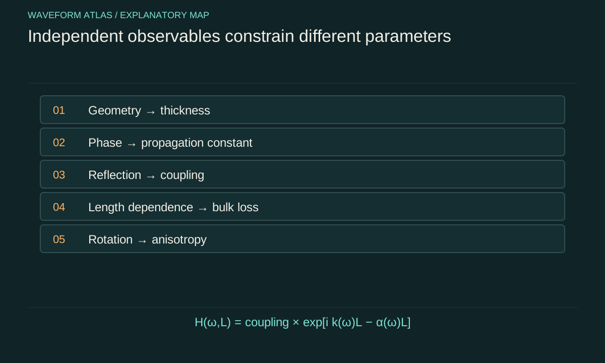
Geometry is part of the material problem

Thickness, surface parallelism, roughness and aperture affect propagation and interference. An error in thickness can be absorbed into a fitted refractive index because both change phase delay. A wedge can spread reflected directions. Roughness can scatter energy outside the detector aperture. These are physical effects of sample geometry, not merely nuisances to subtract without evidence.

Measure geometry independently where possible and propagate its uncertainty into the inferred material parameters. If the sample is nonuniform, state whether the result represents a local measurement, a spatial average or an effective model. A single scalar parameter may be useful operationally while concealing spatial structure that matters in another geometry or at another wavelength.

Amplitude and phase constrain different aspects

Transmission magnitude indicates how much of the selected input reaches a selected output mode. Transmission phase indicates accumulated phase and delay. Reflection adds information about boundary coupling. Together they constrain a model more strongly than any one of them alone. The measurement reference planes must be defined so that external propagation and instrument phase are not mistaken for sample response.

In a lossless ideal layer, a reduced transmitted magnitude can arise from reflection and interference. In an absorbing layer, it can also reflect dissipation. Without reflection or a justified interface model, those contributions may be difficult to separate. The appropriate conclusion is an effective transmission response until additional evidence supports a specific bulk absorption coefficient.

Use multiple lengths to separate interfaces from bulk

Suppose a uniform traveling mode has amplitude proportional to exp(−αL) and phase proportional to kL. Measurements on several lengths can reveal slopes associated with bulk attenuation and phase accumulation, while approximately length-independent coupling factors appear as offsets. This strategy assumes the samples share material properties and comparable interfaces. If fabrication changes with thickness, that assumption must be tested.

As an illustrative calculation, an extra half meter producing an amplitude ratio of 0.9 gives α = −ln(0.9)/0.5, about 0.211 per meter. A phase difference of π over that additional length gives a wavenumber contribution of 2π radians per meter, subject to phase unwrapping. These numbers are model examples. The absolute phase may include additional full cycles that require broadband or other information to resolve.

Frequency sweeps reveal model limits

A narrowband measurement can hide dispersion and resonances. Sweeping frequency tests whether a constant parameter approximation is adequate and reveals phase changes, attenuation peaks and mode cutoffs. The sweep should cover the intended application band with sufficient resolution to resolve narrow features. Averaging too broadly can erase the very structure that limits pulse propagation.

Instrument response must be measured over the same band. A sensor resonance can resemble a material resonance, and a cable or optical path can add phase delay. Use suitable reference measurements and preserve their uncertainty. If calibration becomes unreliable near the edge of the instrument band, do not extend a fitted material curve into that region merely because the plotting software can draw it.

Direction and polarization test anisotropy

Rotate the sample, propagation direction or polarization according to the proposed symmetry. If response changes reproducibly, a scalar isotropic model may be inadequate. The pattern of variation can constrain principal axes and tensor components. Structural information can reduce the number of independent parameters, but the assumed symmetry should be supported by the sample preparation or independent characterization.

Alignment errors matter. A small rotation can mix modes or change coupling, especially near a special axis or degeneracy. Record coordinate conventions and angle uncertainty. When comparing measurements from different orientations, transform quantities into a common basis rather than treating each fitted number as an unrelated material constant. The goal is one model that predicts all orientations consistently.

Amplitude sweeps distinguish regimes

Repeat measurements over a controlled signal range. In a linear regime, the normalized transfer function should remain approximately independent of input amplitude. Deviations can indicate nonlinear response, heating, saturation, structural change or detector nonlinearity. The experiment should identify which explanation is supported rather than label every amplitude dependence an intrinsic fast nonlinearity.

Vary pulse duration or repetition rate when they help distinguish peak-intensity effects from average heating. Allow the sample state to stabilize or model its drift explicitly. A sweep performed only upward can mix amplitude dependence with cumulative changes over time. Reversing the sweep and repeating low-amplitude references helps reveal hysteresis, damage or slow recovery.

Quantify uncertainty and parameter correlation

Fitted parameters often have correlated uncertainties. An increase in thickness may be compensated by a decrease in index, while a change in coupling efficiency may be compensated by attenuation. Report the covariance or a meaningful confidence region when those correlations affect predictions. Independent error bars on each parameter can conceal the directions in parameter space that the data actually constrain.

Use the uncertainty to predict uncertainty in the intended observable. A poorly determined individual parameter may still yield a well-determined delay over the measured band, while extrapolation to another geometry may be highly uncertain. The practical question is whether the characterization supports the proposed application, not whether every fitted coefficient has an impressive number of decimal places.

Reserve an independent prediction

Fit a model using one subset of conditions and test it on another, such as a new thickness, angle, pulse shape or frequency interval. This checks whether the inferred parameters describe the material rather than merely interpolating the calibration data. A failure can reveal missing modes, spatial variation or an invalid effective-medium approximation.

The test should be selected before repeatedly adjusting the model to it. If every new dataset becomes another fitting target, the distinction between calibration and prediction disappears. Updating a model is legitimate, but report that update and seek a further independent comparison. Reproducible predictive performance is stronger evidence than a flexible curve that follows every measurement after its parameters are changed.

Deliver a usable material description

A useful characterization report includes sample preparation, geometry, state variables, frequency and amplitude ranges, measurement reference planes, raw observables, fitted model and uncertainty. It distinguishes directly measured quantities from inferred parameters and records where the model fails. Data outside the supported range should not inherit the same confidence by default.

The purpose is to connect a particular material state to a tested wave response. That connection lets later experiments distinguish ordinary propagation changes from genuinely unexplained residuals. Measuring the medium first does not make the physics less interesting; it provides the baseline needed to decide which features of the outgoing wave require a new explanation.

A minimal dataset can still be deliberately informative

Characterization does not require measuring every conceivable property. It requires enough independent observables to constrain the intended model and its most important alternatives. For a simple single-mode layer, one might combine independently measured thickness with complex transmission and reflection over a limited band. That compact dataset can be more useful than a large collection of intensity-only images taken under nearly identical conditions.

Perform a sensitivity calculation before committing to the measurement. Change each candidate parameter slightly in the forward model and examine how the predicted observables move. If two parameters produce nearly identical changes, the proposed data will struggle to separate them. Add a measurement whose response differs, such as another thickness, incidence angle or polarization. This is an information problem as well as an instrumentation problem.

Finally, preserve the distinction between parameter estimation and model selection. A narrow uncertainty interval within one assumed model does not establish that the model class is correct. Compare residual patterns across frequency and geometry, and test plausible alternative descriptions when the evidence warrants them. The resulting material report can be both concise and honest: a well-constrained effective response over a stated range, with unresolved microscopic interpretations left open rather than assigned false precision.

Reference measurements should be repeated often enough to reveal drift over the experiment. If source output or detector phase changes between calibration and sample acquisition, the inferred material can inherit that drift. Interleaving references provides a direct estimate of this systematic uncertainty and helps distinguish instrumental changes from a genuinely evolving sample.

That reference history should accompany the reported parameter uncertainty.

Go to the original work.

These links identify the sources behind specific claims. Verification scope varies by source and is stated below.

1. 1 / University teachingMIT Physics III: Vibrations and Waves ↗

   Yen-Jie Lee. MIT Physics III: Vibrations and Waves. 2016.

   Wave equations, interfaces, optics and propagation in media.

   Verification scope: MIT course outline inspected; article derivations are independent textbook-level explanations.

2. 2 / University teachingMIT Physics III, Lecture 13: Dispersive Medium, Phase Velocity, Group Velocity ↗

   Yen-Jie Lee. MIT Physics III, Lecture 13: Dispersive Medium, Phase Velocity, Group Velocity. 2016.

   Distinction between phase, group and dispersive pulse propagation.

   Verification scope: MIT lecture page and topic description inspected; no experimental speed is imported.

3. 3 / University teachingFundamentals of Photonics: Wave Propagation in Anisotropic Media ↗

   Franz X. Kärtner. Fundamentals of Photonics: Wave Propagation in Anisotropic Media. 2006.

   Dielectric tensors, polarization eigenmodes, birefringence and energy-flow direction in anisotropic media.

   Verification scope: Direct official PDF and relevant anisotropic wave equations inspected; not a claim of reviewing every example.

4. 4 / University teachingMIT Ultrafast Optics: Lecture Notes ↗

   Franz X. Kärtner. MIT Ultrafast Optics: Lecture Notes. 2005.

   Nonlinear pulse propagation, self-phase modulation, solitons and pulse characterization.

   Verification scope: Official course topic list and relevant textbook excerpt inspected. Illustrative calculations are independently derived.

5. 5 / University teachingTransmission/Reflection and Short-Circuit Line Methods for Measuring Permittivity and Permeability ↗

   J. Baker-Jarvis; M. D. Janezic; J. H. Grosvenor Jr.; R. G. Geyer. Transmission/Reflection and Short-Circuit Line Methods for Measuring Permittivity and Permeability. 1993.

   NIST Technical Note 1355-R: scattering-parameter extraction, reference planes, two-length methods, branch ambiguity and dimensional uncertainty.

   Verification scope: NIST report title page and relevant introduction/method discussions inspected; not all 1355-R equations reread.