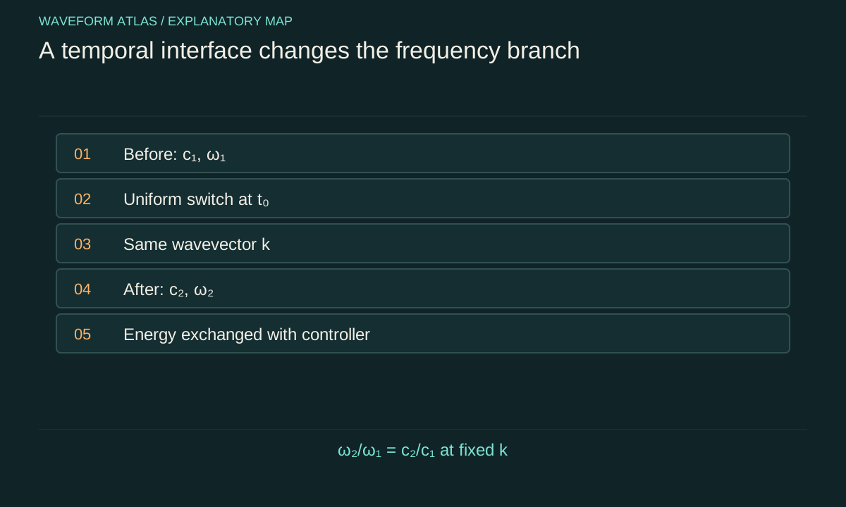
A parameter can change during propagation
Most elementary wave problems assume that material properties remain fixed while a signal passes through. A temporal medium deliberately violates that assumption. Its permittivity, stiffness, capacitance or another constitutive parameter changes while the field is present. The governing equation then has explicit time dependence, and the outgoing field can contain frequencies absent from the input.
This is different from sending a wave through a static spatial gradient. A stationary inhomogeneity preserves time-translation symmetry, so each monochromatic component retains its frequency in a linear model. A temporal change breaks that symmetry. The material controller is an active participant in the energy exchange, even when the modulation is treated as a prescribed function in the wave calculation.
Symmetry identifies the conserved label
If the material changes uniformly throughout an ideal infinite space, spatial translation symmetry remains. A plane-wave component therefore retains its wavevector across the temporal change. Its frequency changes to satisfy the new dispersion relation. This is the temporal counterpart of a stationary spatial interface, where temporal frequency remains fixed while the normal wavevector changes.
The distinction is useful but conditional. A real modulated region has finite size, switches may not act simultaneously, and spatial patterns can exchange momentum with the wave. In such cases wavevector need not be conserved globally. State the actual symmetry of the modulation rather than applying the uniform-time-interface rule to every device with a time-dependent control voltage.
A simple frequency shift has an energy account
Consider an ideal nondispersive scalar model with ω = c_m|k|, where c_m is the medium wave speed. If the speed changes uniformly from c₁ to c₂ while k is retained, the allowed frequency magnitude changes by the ratio c₂/c₁. A twenty-percent speed increase gives a twenty-percent frequency increase for the corresponding branch. This is an original model illustration, not a general optical material formula.
The wave energy need not remain constant because the parameter change can do work on the field. To determine amplitudes and energy transfer, one must apply the correct temporal boundary conditions for the physical variables. Conserving k alone does not determine the full result. The controller, switches or pump must be included when checking whether the total combined energy account closes.
Abrupt and gradual changes differ
An abrupt temporal interface can mix solutions that would be distinct under steady propagation. In a suitable description, forward and time-reflected components appear. A slowly varying change can instead allow an adiabatic evolution of a selected mode, provided the modulation is slow compared with the relevant dynamical timescales and avoids problematic degeneracies.
The word abrupt is relative to the wave period and response times of the medium. A switch that is fast for a low-frequency circuit may be slow for an optical carrier. Material dispersion can also limit how a nominal parameter change is realized. A credible model includes the switching waveform and the bandwidth over which the effective constitutive description remains valid.
Temporal reflection is not an ordinary wall reflection
At a spatial wall, a reflected wave reverses a propagation direction after encountering a localized boundary. At a temporal interface, the material changes over a region at a chosen time, and the field decomposes into solutions of the new dynamics. The resulting reversed temporal ordering or conjugated component has a different origin from a pulse simply bouncing from a stationary surface.
The experiment by Moussa and colleagues reported temporal reflection and frequency translation in a switched transmission-line metamaterial. Its verified abstract describes synchronized switching of effective capacitance. This supports the existence of a specific experimental implementation, not a claim that all materials can be switched instantaneously or that an arbitrary signal can be reversed without limits. Device bandwidth, loss and synchronization remain physical constraints.
Periodic modulation creates sidebands
If a parameter varies periodically at angular frequency Ω, a linear time-periodic system can couple an input frequency ω to sidebands ω + mΩ for integer m. The sideband amplitudes depend on modulation strength, interaction duration, phase and the system response. A spectrum with extra lines can therefore arise from a driven linear system, without requiring an amplitude-dependent material nonlinearity.
This is an important classification point. Time variation and nonlinearity are different properties. A device can be linear in the signal while its coefficients vary in time. Conversely, a time-independent nonlinear medium can mix frequencies because its response depends on field amplitude. Both can produce new frequencies, but their scaling tests and energy sources differ. Varying signal amplitude and modulation parameters helps distinguish them.
Modulation phase can control interference
When several conversion pathways lead to the same output mode, their relative phases affect the result. Two temporal interfaces can produce interference analogous in structure to multiple spatial interfaces. The interval between switches determines accumulated phase, while switch strength determines coupling amplitudes. A frequency-converted output can increase or decrease as that interval changes.
The effect is not automatically gain. Interference can redirect energy among modes while the modulation also exchanges energy with the field. A complete measurement resolves the output spectrum and, where relevant, direction. Summing only the original-frequency channel can make conversion look like absorption. Summing only one enhanced channel can make redistribution look like unlimited amplification.
Stability constrains useful operation
Periodic parameter variation can produce parametric amplification or instability in suitable regimes. The modulation transfers energy into the wave when the phase and frequency relationships permit it. Loss competes with that input. A small-signal model can predict exponential growth only within the range where the prescribed parameters and linear response remain valid.
As amplitude grows, saturation, heating, nonlinear response or controller limits can change the dynamics. A design should therefore assess stability, transient behavior and the energy demanded from the pump. An ideal mathematical gain curve is not a complete operating specification. The useful device must remain controlled for the expected input levels and disturbances, including the case of no intended signal but unavoidable noise.
Measure the control as well as the field
Record the actual switching or modulation waveform at the relevant location, not only the command sent to a controller. Timing skew across a spatial array can create an unintended traveling modulation. Finite switching edges can change conversion efficiency and generate additional spectral content. These effects can explain departures from an ideal uniform temporal model.
Measure input and output spectra with calibrated phase and amplitude where feasible, and compare modulation-on with modulation-off conditions. Track energy delivered by the control circuit or pump when making energy-balance claims. A frequency shift consistent with a temporal model is stronger evidence when the independently measured parameter change predicts its size and when competing spatial-scattering effects are constrained.
State the space–time approximation explicitly
A useful temporal-medium result identifies the changed parameter, modulation waveform, spatial extent, signal bandwidth and material response time. It states which symmetry argument is used and which outgoing modes are measured. If a simple effective model describes a complex switched structure, its validity range should accompany the inferred parameters.
The central mechanism is controlled exchange between a wave and a changing environment. Frequency conversion, temporal reflection and parametric gain can follow from that exchange under different conditions. None implies energy creation from nothing or a suspension of ordinary evolution. The controller supplies the missing part of the physical story, and the measured space–time dependence determines which conservation statements remain applicable.
Check work done by a changing oscillator parameter
A single harmonic oscillator provides a compact analogy for temporal material control. Let its energy be E = p²/(2m) + K(t)x²/2 with fixed mass and a time-dependent spring constant. Along its ideal motion, the explicit parameter change contributes dE/dt = (1/2)(dK/dt)x². Increasing stiffness while displacement is nonzero supplies energy; changing it near a displacement zero has a different immediate effect. The modulation phase therefore matters.
For an instantaneous ideal stiffness change from K₁ to K₂, position and momentum remain continuous if no separate impulsive force is applied. The energy changes by (K₂ − K₁)x²/2 at that instant. This calculation is an original mechanical illustration, not a replacement for electromagnetic temporal boundary conditions. It makes visible how a prescribed parameter change can transfer work without violating conservation in the larger system.
The analogy also cautions against characterizing modulation only by its average value. Two schedules with the same average stiffness can deliver different net work because they act at different phases of the motion. In a wave device, the timing, spatial pattern and phase of the control similarly affect conversion and gain. Measuring the control waveform is therefore part of measuring the interaction, rather than an optional engineering detail appended after the field behavior has been explained.
Finite modulation regions also have entrance and exit boundaries. Reflections from those boundaries can overlap the temporally converted signal. A reference run with identical geometry and no switching helps isolate this contribution before the temporal-interface model is evaluated.
What to take forward
- Time variation can change frequency by exchanging energy with a controller.
- Wavevector conservation requires spatially uniform modulation.
- Time-periodic linear conversion is distinct from amplitude-dependent nonlinearity.
Go to the original work.
These links identify the sources behind specific claims. Verification scope varies by source and is stated below.
- 1 / Primary researchObservation of temporal reflection and broadband frequency translation at photonic time interfaces ↗
H. Moussa; G. Xu; S. Yin; E. Galiffi; Y. Ra’di; A. Alù. Nature Physics 19, 863–868 (2023).
DOI: 10.1038/s41567-023-01975-y
Switched transmission-line experiment demonstrating temporal reflection and broadband frequency translation; the medium is actively changed.
Verification scope: Publisher bibliographic record and abstract inspected
- 2 / Primary researchPhotonics of time-varying media ↗
E. Galiffi; R. Tirole; S. Yin; H. Li; S. Vezzoli; P. A. Huidobro; M. G. Silveirinha; R. Sapienza; A. Alù; J. B. Pendry. Advanced Photonics 4(1), 014002 (2022).
Review of temporal switching, time interfaces, spatiotemporal modulation and amplification.
Verification scope: Publisher record and abstract inspected; detailed derivations not reread
- 3 / University teachingMIT Physics III: Vibrations and Waves ↗
Yen-Jie Lee. MIT Physics III: Vibrations and Waves. 2016.
Wave equations, interfaces, optics and propagation in media.
Verification scope: MIT course outline inspected; article derivations are independent textbook-level explanations.
Found a problem with a claim or calculation? Send the page, the claim and the evidence. Read how these articles were prepared.