A medium that changes from place to place

A medium can vary without a sharp boundary

A material property may change continuously with position. Examples include a refractive-index profile, a sound-speed gradient or a string whose mass per length varies. The wave then encounters a sequence of local environments rather than one abrupt junction. Its phase and amplitude evolve according to the spatially varying equation and the boundary conditions of the entire structure.

The relevant comparison is between the scale over which properties change and the local wavelength. A gradient that is gentle for a short wavelength can be abrupt for a long one. Calling a profile smooth by visual inspection is not enough. Quantify its variation relative to the wave's spatial scales before choosing a ray, slowly varying or full-field description.

Local phase defines a wavevector

In a slowly varying approximation, write a field as an amplitude multiplied by an oscillating phase. The gradient of that phase is the local wavevector. The material's local dispersion relation connects this wavevector to frequency. A stationary medium preserves temporal frequency for each monochromatic component, while spatial variation changes its local wavelength and propagation direction.

For an isotropic optical index n(r), the local wavenumber magnitude is approximately n(r)ω/c. Rays follow the resulting phase geometry under the approximation's conditions. This description is powerful when the amplitude and medium vary slowly over a wavelength. It becomes unreliable near points where the amplitude changes rapidly, rays cross or an allowed propagating branch ends.

A transverse gradient bends a ray

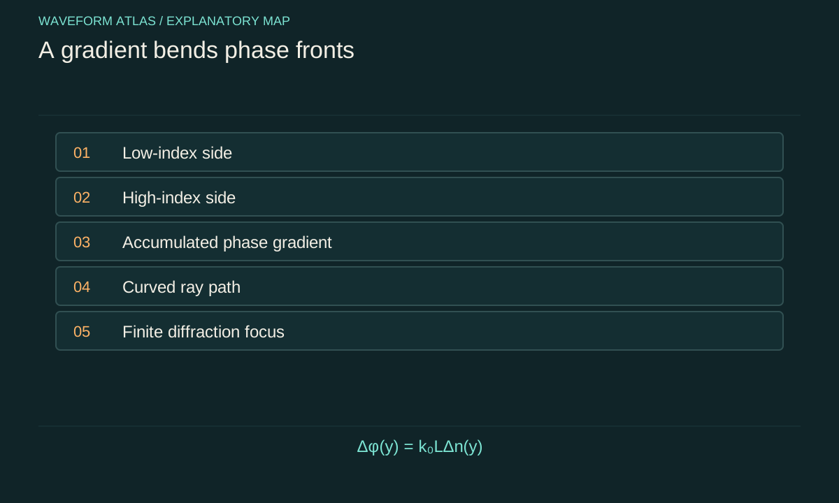
A planar wave crossing a region with a higher index on one side accumulates phase more rapidly there. The phase front tilts, and the propagation direction bends. In ray language, the path curves toward regions of higher index under ordinary isotropic conditions. The precise curvature follows the index gradient and the chosen geometry, not merely the value of index at the starting point.

A simple thin-element illustration makes the phase effect explicit. A slab with thickness L and a small transverse index variation Δn(y) adds phase Δφ(y) = k₀LΔn(y). A linear phase gradient deflects a beam, while a quadratic phase profile can focus or defocus it in the paraxial approximation. The finite aperture and diffraction determine the final spot size and side structure.

Longitudinal gradients can reduce reflection

If impedance changes gradually along the propagation direction, a wave can adapt with less reflection than at a sudden jump. This is the idea behind a taper or graded matching region. The improvement depends on how slowly the relevant propagation parameters vary, the available length and the spectrum of the input. A gradient is not automatically reflectionless.

One common local criterion in a scalar wave model is |dk/dx| much smaller than k². It compares the change of wavenumber over one wavelength with the wavenumber itself. Near k = 0 the criterion fails even if the underlying material profile is smooth. Such turning points require special treatment and can produce strong reflection. The mathematical failure is physically meaningful, not just a numerical inconvenience.

Turning points separate propagation from evanescence

In a guided or cutoff system, a local propagation constant can decrease to zero and become imaginary beyond a certain location. The wave then reaches a turning region rather than continuing as an ordinary traveling mode. A slowly varying approximation based on a nonzero local wavenumber breaks down there. Reflection and an evanescent continuation must be described consistently.

This behavior should not be called absorption unless energy actually enters dissipative channels. A field can decay spatially in a forbidden region while the incident energy is reflected. A second nearby allowed region can permit tunneling-like transmission in an appropriate wave model. The spatial decay length, barrier width and boundary matching determine that outcome, not an assumption that decaying amplitude always means lost energy.

Focusing changes amplitude through geometry

When rays converge, energy is concentrated into a smaller area and amplitude can increase without an active gain source. When rays diverge, amplitude can decrease without dissipation. A flux account must include the changing cross-sectional area of the ray bundle. Comparing two local amplitudes without this geometry can misidentify focusing as amplification or spreading as absorption.

At a geometrical focus, simple ray theory can predict an unphysical divergence. Diffraction and finite aperture resolve it. A full wave calculation produces a finite focal pattern with a characteristic width and side structure. The medium's gradient determines the phase transformation, while wavelength and aperture constrain the achievable concentration. These are complementary parts of the same explanation.

Disorder is a different spatial variation

An inhomogeneous medium can contain random fluctuations rather than a designed smooth gradient. Small-scale variations scatter waves into other directions and modes. Their effect depends on correlation length, strength and wavelength. A mean index profile may describe average refraction while missing scattering from the fluctuations around that mean.

Measure or model both the average and the spatial statistics when they matter. Two samples with the same mean property can have different transport because their fluctuation spectra differ. A narrow forward detector cannot distinguish all these possibilities. Angular scattering and spatial coherence measurements can reveal whether the apparent attenuation arises from disorder rather than from the smooth background gradient.

Frequency changes the path through one profile

If the material is dispersive, the spatial index profile can differ across frequency. A broadband pulse can then experience both temporal dispersion and frequency-dependent bending or focusing. Even when each frequency follows a well-defined ray approximation, the combined pulse may separate spatially or distort at the detector. A design optimized for one color or tone may perform poorly for a wide spectrum.

Characterize the profile over the actual bandwidth and include the detector aperture in the prediction. A pulse can appear attenuated because some frequencies are focused elsewhere, not because they were absorbed. Measuring the output field across space and frequency separates this spatial filtering from true bulk loss. The relevant output mode must be defined before assigning an efficiency.

Inverse reconstruction is often nonunique

A measured travel time constrains an integral of slowness along a path. Different spatial profiles can produce the same total delay. A single transmitted intensity adds another constraint but may still leave many possibilities. Multiple paths, frequencies or boundary conditions help reconstruct the profile, provided the forward model is appropriate.

Do not interpret a successful fit to one arrival time as a unique map of the medium. Report the parameterization, prior structural information and resolution of the reconstruction. Fine features smaller than the measurement sensitivity can remain unresolved. A physically meaningful uncertainty map is more informative than a detailed-looking profile whose apparent precision comes mainly from the chosen fitting basis.

Design with the full path in mind

A useful graded medium is specified by a profile, length, aperture and operating band. Its performance should be evaluated in terms of reflected flux, transmitted mode, phase distortion and tolerance to fabrication or temperature changes. A smoother profile may reduce reflection but require more length, allowing more absorption or accumulating unwanted dispersion.

The central mechanism is continuous adaptation of phase and amplitude to a spatially changing propagation law. That mechanism can bend, focus, spread or reflect a wave without invoking a change in fundamental dynamics. The strongest explanation identifies the scale separation supporting its approximation and checks the places where that approximation is most likely to fail.

A gradient must be resolved by the measurement too

Suppose the local wavenumber varies over a characteristic length L_g. The slowly varying condition is roughly that many wavelengths fit within L_g, with additional care near zeros or resonances. A sensor array with spacing larger than L_g may nevertheless report an apparently abrupt change because it cannot resolve the gradient. The approximation used for the physics and the resolution used for observation are separate scale comparisons.

Choose sensor spacing that resolves both the phase and the property variation relevant to the model. Too-large spacing creates phase ambiguity, while too-small spacing can make phase differences difficult to measure accurately against noise. Multiple separations can help balance these limitations. When reconstructing a profile, report spatial resolution rather than only the grid spacing used by the numerical solver; a fine computational grid does not create new experimental information.

An original thought experiment illustrates the ambiguity. Two smooth profiles can have the same integrated optical path and therefore the same normal-incidence phase delay, while one contains a transverse gradient that deflects the beam and the other does not. Measuring only delay cannot distinguish them. Adding an output-angle measurement resolves that particular ambiguity. This is the general pattern in inhomogeneous-media problems: select observables that respond differently to the competing spatial structures, instead of expecting one global number to reveal the entire medium.

A useful validation changes the source position while retaining the same medium. A reconstructed spatial profile should predict the altered path or field without being refitted from scratch. Agreement tests spatial information that a single original trajectory could not constrain.

Go to the original work.

These links identify the sources behind specific claims. Verification scope varies by source and is stated below.

1. 1 / University teachingMIT Physics III: Vibrations and Waves ↗

   Wave equations, interfaces, optics and propagation in media.

   Verification scope: MIT course outline inspected; article derivations are independent textbook-level explanations.

2. 2 / University teachingMIT Physics III, Lecture 13: Dispersive Medium, Phase Velocity, Group Velocity ↗

   Distinction between phase, group and dispersive pulse propagation.

   Verification scope: MIT lecture page and topic description inspected; no experimental speed is imported.