Different frequencies, different propagation

A pulse contains a spectrum

A localized pulse cannot be described by one exact frequency. It is a superposition of spectral components with particular amplitudes and phases. A linear time-independent medium acts on each component through a transfer function H(ω). The output spectrum is H(ω) times the input spectrum. Both the magnitude and phase of H matter when those components are recombined into a time-domain waveform.

If the magnitude is unity across the pulse bandwidth but the phase varies nonlinearly with frequency, the pulse can change shape while conserving its spectral energy in the ideal model. If the magnitude varies, the medium also filters the spectrum. Measuring only the output peak cannot distinguish these effects. A smaller peak can result from spreading the same energy over a longer interval.

Expand the propagation constant locally

For propagation through a uniform length L, the spectral phase includes k(ω)L. Around a carrier frequency ω₀, expand k as k₀ + k₁Ω + k₂Ω²/2 plus higher terms, where Ω = ω − ω₀. The constant term sets a carrier phase. The linear term shifts the envelope in time by k₁L. The quadratic term introduces group-delay dispersion and changes the relative timing of spectral components.

This expansion is useful only over a bandwidth where the retained terms describe k accurately. A broad pulse near a resonance may require higher derivatives or the full measured transfer function. Truncating the series because a quadratic model is convenient can hide asymmetric tails, satellite pulses or other distortions. The model order should be tested against the actual input spectrum and measured material response.

Phase and group velocity answer different questions

Phase velocity is ω/k and describes motion of a constant-phase surface. Group velocity is 1/(dk/dω) for a narrowband packet under suitable conditions. They coincide in a nondispersive medium with a linear relation between k and ω through the origin. In a dispersive medium they generally differ, and neither should be inferred from the other without checking the derivative.

The group-velocity picture is most reliable when the pulse remains recognizable and the bandwidth is narrow enough for the linear term to dominate its delay. Strong filtering or rapid phase variation can move the output peak by reshaping it. A peak advance then need not represent a signal or energy traveling at that apparent speed. The complete input–output relation is safer than a single peak-tracking number in such regimes.

A Gaussian example makes broadening quantitative

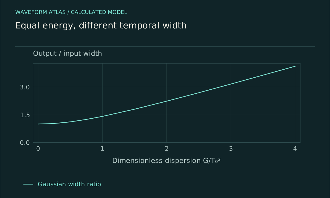
Let the input field envelope be exp[−t²/(2T₀²)], and let the medium add only quadratic spectral phase with G = k₂L. In the ideal lossless model, the output intensity width parameter becomes T = T₀√[1 + (G/T₀²)²]. The field also acquires a time-dependent phase, often described as chirp. The total pulse energy is preserved even though peak intensity decreases.

If G = T₀², the width increases by √2 and the peak intensity falls by 1/√2 for fixed energy and the same Gaussian convention. If G = 3T₀², the width factor is √10, about 3.162. These are original model calculations. State whether width means the Gaussian parameter, standard deviation or full width at half maximum before comparing it with a plotted measurement.

Chirp can be reversed under controlled conditions

If one element adds a quadratic spectral phase G and another adds −G over the relevant bandwidth, the ideal combined phase cancels. A broadened pulse can recompress. This illustrates why dispersive spreading is not automatically irreversible dissipation. The information about spectral phase remains in the field, provided loss, noise and uncontrolled distortions have not removed it.

Practical compensation is limited by bandwidth and higher-order phase. A device that cancels k₂ at the carrier can leave cubic or more complicated contributions. Spectral amplitude filtering cannot generally be undone by a passive phase-only element. Report both the recovered pulse shape and throughput. A narrow recovered peak accompanied by large energy loss is a different result from efficient restoration of the original mode.

Initial chirp changes the outcome

A pulse can enter the medium already carrying a frequency-dependent phase. Added dispersion can then broaden or compress it depending on the sign and magnitude relative to the initial chirp. The same material may make one input longer and another shorter. A claim that a medium always broadens pulses is therefore too broad unless the input phase is specified.

This dependence is experimentally useful. Preparing known input chirps and measuring output widths can constrain the material's dispersive phase. However, intensity width alone may not uniquely determine the phase because different pulse shapes can share the same width. A phase-sensitive pulse characterization or a carefully justified model is needed when the full waveform matters.

Absorption and dispersion often coexist

Real material resonances affect both phase response and attenuation. It is therefore common for a strongly dispersive band to have significant loss or gain. The ideal all-pass example separates mechanisms for clarity, not because every material offers large dispersion without any amplitude change. A measured transfer function should include both parts.

The distinction remains valuable even when they coexist. Spectral attenuation removes or redirects energy from selected components, while spectral phase changes how retained components interfere in time. Their contributions can be estimated separately from calibrated amplitude and phase data. This prevents an observed long output tail from being assigned wholly to slow transport when some of its shape arises from filtering or resonant storage.

Spatial dispersion creates related effects

Dispersion is not limited to optical pulses. Water waves, elastic waves and guided modes can have nonlinear frequency–wavenumber relations. Different wavelengths in a localized disturbance then travel differently. A wave packet can spread, and its phase crests can move through the envelope. The material, geometry and boundary conditions jointly determine the dispersion relation.

For deep-water gravity waves in an ideal inviscid model, ω² = gk, so group velocity is half phase velocity. This is a specific regime, not a general water-wave identity. Finite depth, surface tension or an elastic cover change the relation. The example reinforces the method: differentiate the actual dispersion law rather than import a velocity ratio from a visually similar wave.

Measure the complex transfer function

A broadband input and calibrated output can reveal amplitude and phase versus frequency. The reference path, sensor response and sample length must be known. Multiple lengths help separate bulk propagation from interface effects. When signal levels are low, phase estimates become unstable, so uncertainty should accompany regions of strong attenuation.

Time-domain measurements are complementary. Compare integrated energy, peak height, width, asymmetry and delayed components. A pulse that broadens with nearly unchanged integrated energy supports a different interpretation from one whose entire spectrum is attenuated. The observation window must be long enough to collect the broadened tail; otherwise energy spreading can be misreported as loss simply because the integration ends too early.

Describe the transformation rather than one speed

A complete dispersive result states the input spectrum and phase, the material transfer function or fitted derivatives, the propagation length and the measured output. It identifies whether the dominant effect is delay, chirp, broadening, compression, filtering or a combination. The chosen summary should match what the data can resolve.

This approach replaces the vague statement that the wave slowed down with a testable account of its components. Some phases advance differently, the envelope can reshape, and energy can remain conserved within the ideal model. When loss is present, it receives its own account. Dispersion is fundamentally a relationship between frequency and propagation, not a synonym for damping or destruction.

Use a dimensionless dispersion strength

For the Gaussian model, define s = G/T₀². The broadening factor is √(1 + s²), so the same material length affects short pulses more strongly than long ones. Halving T₀ increases |s| by a factor of four when G is fixed. A device that leaves a long pulse nearly unchanged can therefore substantially distort a pulse with half the duration, even though both have the same carrier frequency.

This scaling provides a direct experimental test. Prepare pulses with known input widths and phases, propagate them through the same element, and compare the measured broadening with the predicted dependence on T₀. If the data depart systematically, possible explanations include higher-order dispersion, non-Gaussian input shape, initial chirp, nonlinear phase or spectral filtering. The discrepancy guides the next model refinement rather than automatically invalidating the concept of dispersion.

The energy check is separate. In the ideal lossless calculation, the area under intensity remains constant while the peak changes inversely with width. If the measured area decreases, investigate coupling, absorption, scattering or a recording window that misses the tail. If the area increases, an active energy source or calibration issue must be considered. Comparing width, peak and integrated energy together supplies three linked tests of a simple model and makes a pulse transformation much harder to misclassify from one visually striking trace.

Go to the original work.

These links identify the sources behind specific claims. Verification scope varies by source and is stated below.

1. 1 / University teachingMIT Physics III, Lecture 13: Dispersive Medium, Phase Velocity, Group Velocity ↗

   Yen-Jie Lee. MIT Physics III, Lecture 13: Dispersive Medium, Phase Velocity, Group Velocity. 2016.

   Distinction between phase, group and dispersive pulse propagation.

   Verification scope: MIT lecture page and topic description inspected; no experimental speed is imported.

2. 2 / University teachingMIT Physics III: Vibrations and Waves ↗

   Yen-Jie Lee. MIT Physics III: Vibrations and Waves. 2016.

   Wave equations, interfaces, optics and propagation in media.

   Verification scope: MIT course outline inspected; article derivations are independent textbook-level explanations.

3. 3 / University teachingMIT Ultrafast Optics: Lecture Notes ↗

   Franz X. Kärtner. MIT Ultrafast Optics: Lecture Notes. 2005.

   Nonlinear pulse propagation, self-phase modulation, solitons and pulse characterization.

   Verification scope: Official course topic list and relevant textbook excerpt inspected. Illustrative calculations are independently derived.

4. 4 / University teachingFundamentals of Photonics, Chapter 2: Classical Electromagnetism and Optics ↗

   Franz X. Kärtner. Fundamentals of Photonics, Chapter 2: Classical Electromagnetism and Optics. 2006.

   §§2.1.6–2.1.8: group velocity, Gaussian broadening and complex index; §§2.2.1–2.2.5: boundary phase matching, flux coefficients and total internal reflection; §2.3: multilayers.

   Verification scope: Relevant PDF passages inspected; uses exp(+jωt), opposite to the article’s exp(−iωt) loss-sign convention.