Reversibility as a diagnostic

Begin with an operation you can define

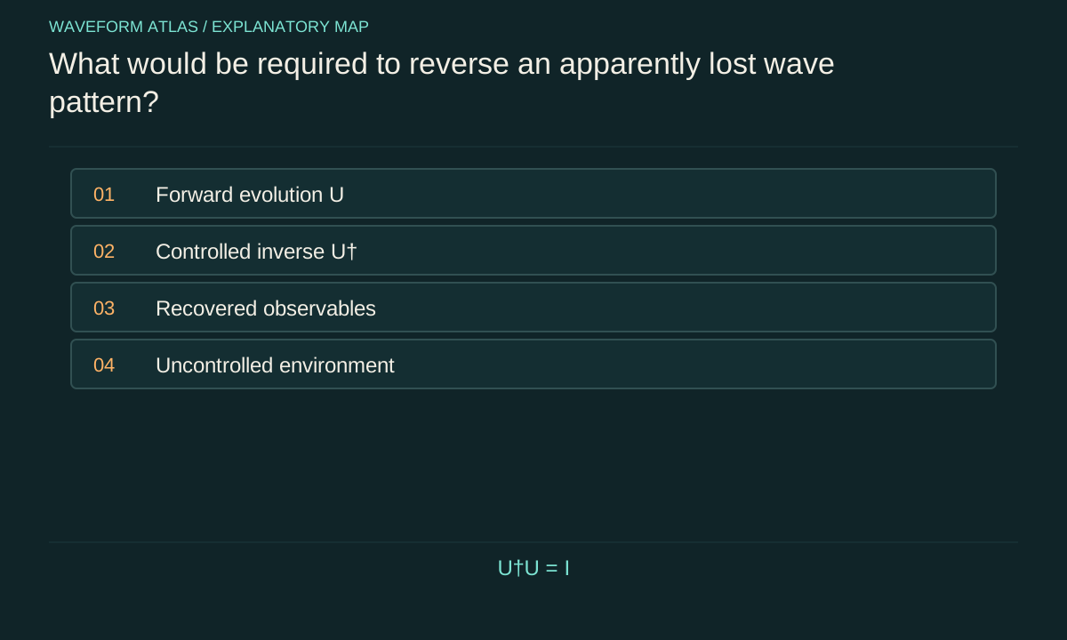
A closed quantum system evolves unitarily in the standard model. If the forward evolution is U, its mathematical inverse is U†, and applying U†U restores the initial state. This statement is exact within the model. It does not imply that an experimentalist can implement the inverse easily, or that simply waiting for the same duration applies it. Another interval under the same Hamiltonian generally continues the forward evolution.

For a time-independent Hamiltonian H, U(t) = exp(−iHt/ℏ), while U†(t) = exp(+iHt/ℏ). Engineering the latter requires an appropriate control sequence or effective reversal of the relevant dynamics. The distinction between existence of an inverse and practical access to it is central. A spreading or scrambled pattern can be reversible in principle while demanding control far beyond what the apparatus can achieve.

Time-reversal symmetry is a separate statement

Time reversal as a physical symmetry compares a process with one in which time-odd quantities, such as momenta, are appropriately reversed. In quantum mechanics the symmetry is represented by an antiunitary transformation, with additional structure for spin. It is not merely multiplication by U†, nor is it generally implemented by playing a movie backward. Whether a particular Hamiltonian respects that symmetry depends on the physical interactions and external fields.

The present discussion does not assume that every fundamental interaction is time-reversal invariant. Its practical focus is narrower: can the evolution relevant to a particular wave experiment be inverted or refocused under a specified model? A system can admit an engineered inverse over a controlled interval without resolving every question about microscopic time-reversal symmetry. Keeping the concepts separate prevents an ordinary echo experiment from being overstated as a reversal of time itself.

Undo deterministic phase dispersion

Suppose an ensemble of qubits has static frequency offsets δω during each run. Under H = ℏδωσz/2, different members accumulate different phases and the average transverse signal falls. An ideal inversion pulse X changes the sign of σz in the toggling frame. Free evolution for a time τ, followed by X and another equal free interval, refocuses the static phase offsets, up to the known pulse action.

A suitable final rotation or readout convention accounts for that remaining action. The recovered echo shows that the apparent signal loss arose from phase dispersion accessible to the control sequence. It does not mean every environmental effect was undone. The calculation assumes offsets remain effectively static during the sequence and pulses are accurate and fast enough. If those conditions fail, incomplete recovery can occur within ordinary dynamics.

Distinguish refocusing from reversing all interactions

An echo targets a particular class of phase errors. It may reverse an inhomogeneous frequency distribution while leaving energy relaxation, rapidly varying noise and unwanted couplings largely untouched. Therefore the echo amplitude is a diagnostic of the noise filtered by that sequence, not a universal measure of all information lost from the system. Different pulse patterns can yield different recovery times because they address different spectral components.

This is why a successful echo is stronger evidence for a specific reversible contribution than a failed echo is for fundamental irreversibility. Failure has many explanations: pulse errors, drifting offsets, environmental records, absorption or a wrong Hamiltonian model. A credible experiment calibrates its recovery operation on known cases and quantifies those conventional limitations before drawing conclusions about an additional collapse mechanism.

Reverse dispersion with a matching phase

A coherent wavepacket can spread because its spectral components acquire a deterministic quadratic phase. If a device applies the opposite spectral phase over the occupied bandwidth, the original envelope can be restored in an ideal model. The spectrum’s magnitude need not have changed during the spreading. This is a concrete example of a familiar shape disappearing while the information needed to reconstruct it remains in the field.

Recovery of intensity alone is not always sufficient to establish full state recovery. Two packets can have the same spatial width but different phase chirps or correlations. A phase-sensitive measurement or a later propagation test can distinguish them. The recovery target should match the task: restoring a pulse’s peak, its full complex envelope and an arbitrary quantum state are different achievements with different calibration demands.

Include the environment in the bookkeeping

If a system becomes entangled with an environment, reversing only the system’s local evolution may not restore the original state. Information about its alternatives can remain in scattered photons, gas particles or internal modes. In a fully unitary description, an inverse on the entire system–environment state exists mathematically, but implementing it requires controlling those correlations as well. The practical obstacle can be enormous.

The partial trace used to describe the subsystem does not itself destroy the global information. It acknowledges that the experiment does not access the environment. This distinction explains why a locally mixed state can arise through reversible global dynamics. It also clarifies the experimental challenge for objective-collapse tests: ordinary inaccessible correlations can produce apparent irreversibility, so a failure of local recovery does not uniquely establish a new fundamental reduction process.

Quantify recovery rather than inspect resemblance

A recovery experiment should compare measurable properties of the restored state with the initial preparation. For a known pure target, fidelity F = ⟨ψ0|ρrecovered|ψ0⟩ is one useful quantity if it can be estimated under a calibrated measurement model. Other tasks may use recovered contrast, waveform overlap or restored correlations with a reference system. Each metric has a defined scope.

A high overlap in one intensity trace does not guarantee that entanglement with a reference was preserved. Conversely, a modest-looking local signal may still retain useful correlations. Choose the metric before interpreting the experiment, and include uncertainty from preparation and readout. If the inverse operation itself has limited fidelity, separate that limitation from the forward process when possible. Otherwise an imperfect recovery may be assigned to the wrong stage.

Chaotic sensitivity makes reversal demanding

In a many-degree-of-freedom system, small control errors can grow under the dynamics. Reversing an ideal trajectory may require extraordinarily precise knowledge of phases and momenta. This sensitivity helps explain why macroscopic reversals are difficult even when an underlying model is reversible. It does not turn an inaccurate inverse into evidence that the original evolution lacked an inverse.

The relevant experimental question is how recovery degrades as the deliberately introduced reversal error is varied. A reproducible dependence can reveal sensitivity to perturbations and unmodeled couplings. The result should be interpreted within the controlled system and observable. A dramatic failure to reconstruct a complex wave field may reflect practical limits of phase control rather than an additional law that erases information after a particular duration.

Recovery can constrain a collapse claim

A model predicting irreversible destruction of a specified coherence can be tested by preparing that coherence, allowing the proposed process to act and attempting a calibrated recovery. If the relevant coherence returns beyond what the model allows, the model or its parameter choice is constrained. The comparison must use the model’s quantitative prediction and the actual preparation, rather than treating any recovered signal as a universal refutation of all collapse ideas.

A null recovery is less decisive unless conventional explanations are tightly bounded. Loss, detector acceptance, imperfect inversion and ordinary decoherence may all suppress the same observable. Secondary predictions such as heating or radiation can provide additional discrimination for some models. The strongest test combines a well-characterized inverse with independent observables and parameter changes that make the competing explanations diverge.

State what was reversed and what was measured

A clear report names the forward Hamiltonian or channel, the attempted inverse, the controlled degrees of freedom and the recovery metric. It identifies which environmental interactions were included and which were inaccessible. It distinguishes time-reversal symmetry from an engineered echo and both from a reversed video. These statements allow another researcher to calculate the expected recovery and locate possible errors.

Reversibility is useful because it asks where the information about a pattern went. A successful inverse can show that a change was coherent and recoverable within the tested model. An unsuccessful inverse identifies a problem to diagnose, not automatically a fundamental destruction mechanism. By tying reversal to explicit operations and observables, the experiment turns an abstract question about time into a practical test of dynamics, control and the limits of the chosen description.

Purity provides another useful diagnostic in a controlled qubit example. A dephased |+⟩ state with coherence factor c has purity (1+c²)/2. For c = 0.8, that is 0.82. No unitary acting on that qubit alone can raise the purity to one, because a unitary preserves the density operator’s eigenvalues. Recovery would require additional information, an auxiliary resource or a nonunitary operation, rather than a simple local phase rotation. By contrast, an unknown but fixed coherent rotation preserves purity and can be undone once identified. The distinction helps separate coherent miscalibration from mixedness in a state estimate. It does not reveal whether the mixedness arose from a classical ensemble or entanglement with an inaccessible environment without further measurements.

Go to the original work.

These links identify the sources behind specific claims. Verification scope varies by source and is stated below.

1. 1 / University teachingPreskill, Quantum Information, Chapter 3: Measurement and Evolution ↗

   Measurement operators, channels, dephasing, amplitude damping and open-system evolution.

   Verification scope: Author-hosted lecture PDF inspected for relevant sections; not an exhaustive audit of every lecture derivation.

2. 2 / University teachingMIT OpenCourseWare, Quantum Physics I (2016), lecture notes ↗

   Schrödinger evolution, stationary states, Fourier wavepackets, observables and time delay.

   Verification scope: Official course notes index and named lesson records inspected; articles provide original elementary derivations.

3. 3 / University teachingMIT OpenCourseWare, Time evolution of a free particle wavepacket ↗

   Free-particle wavepacket evolution as distinct from loss or measurement.

   Verification scope: Official lesson record inspected; formula and numerical examples independently checked algebraically.

4. 4 / Primary theoryZurek, Decoherence, einselection, and the quantum origins of the classical ↗

   Environmental monitoring, preferred records and suppression of local interference.

   Verification scope: Author-posted review abstract and bibliographic record inspected.

5. 5 / University teachingPreskill, Quantum Information, Chapter 2: States and Ensembles ↗

   Density operators, composite states, measurement probabilities, quantum erasure and local statistics.

   Verification scope: Author-hosted lecture PDF inspected for relevant foundational definitions; independent elementary examples are worked in the article.

6. 6 / University teachingMIT OpenCourseWare, Statistical Mechanics I (2013), lecture notes ↗

   Liouville evolution, Boltzmann’s equation, the H-theorem and their assumptions.

   Verification scope: Official course notes index inspected, including the named irreversibility and conservation-law lessons.

7. 7 / Primary theoryBassi et al., Models of Wave-function Collapse, Underlying Theories, and Experimental Tests ↗

   Research authors’ synthesis of stochastic collapse dynamics, motivation and distinct experimental signatures.

   Verification scope: Author-posted review abstract and bibliographic record inspected; general equations below are explicitly specified teaching models.