A lifetime describes a specific unstable preparation

Define the preparation whose survival is counted

A lifetime is meaningful only after the unstable preparation is named. It might be an excited atomic level, a metastable mechanical excitation, a particle species or a population difference in a two-level system. The event counted as leaving that preparation must also be defined. Emission into a particular detector is not always identical to total decay, because some channels may be unobserved or nonradiative.

The time origin is part of the definition. It may be a preparation pulse, a particle-production event or a herald. If the preparation has finite duration, the observed distribution can be a convolution of creation times and survival dynamics. A precise clock does not remove that uncertainty automatically. The model should connect the physical preparation to the timing record before a fitted slope is interpreted as a property of the unstable state.

Write the survival probability

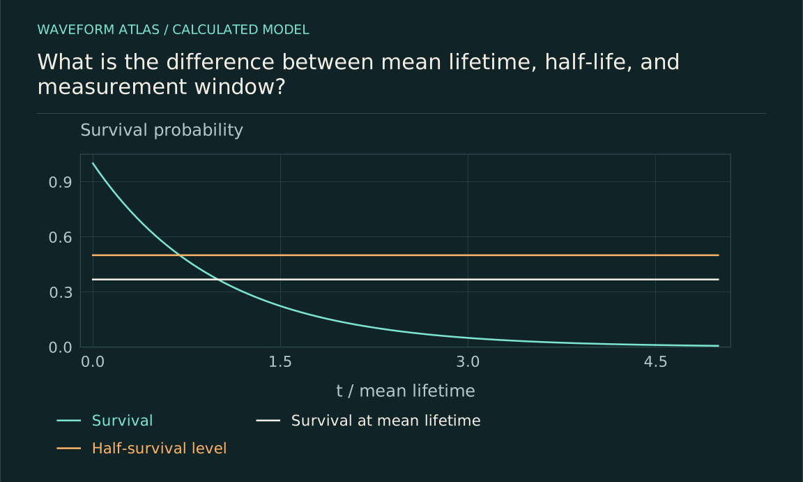
Let S(t) be the probability that the specified preparation survives to time t. In a constant-rate model, dS/dt = −ΓS with S(0) = 1, giving S(t) = exp(−Γt). The event-time probability density is f(t) = Γexp(−Γt). These are different functions: S is dimensionless, while f has units of inverse time. A histogram of decay times estimates the latter after binning and detector effects.

The mean event time is τ = 1/Γ. The probability of surviving one mean lifetime is e⁻¹, about 0.368, so the mean is not a deadline by which every member has decayed. Exponential waiting times have a long tail. An individual event occurring after several lifetimes is possible; its rarity is quantified by S(t), not forbidden by the definition of the mean.

Half-life is a median in the exponential model

The half-life satisfies S(t1/2) = 1/2, so t1/2 = ln 2/Γ = τ ln 2. It is shorter than the mean lifetime. After one half-life, half the initial ensemble survives on average; after two, one quarter survives. These statements concern expected fractions for repeated preparations or large ensembles, not exact counts in every small sample.

If τ = 10 microseconds in a teaching example, the half-life is about 6.93 microseconds. At 20 microseconds, the survival probability is e⁻², about 0.135. Mixing these quantities can create large errors in experimental planning. A detector window of ten microseconds captures about 63.2% of ideal decay events from an instantaneous preparation, not all of them and not exactly half. The intended fraction should be calculated from the stated model.

A measurement window is an instrumental choice

An observation window limits which events are recorded. If the window ends before some preparations decay, those trials are right-censored rather than known to have infinite lifetime. If events before a start threshold are excluded, the sample is left-truncated. These selection rules change the likelihood used to estimate a lifetime. Ignoring them can bias the result even when the underlying dynamics are exactly exponential.

For an exponential process, the conditional distribution after surviving to a later start time retains the same rate, reflecting memorylessness. A finite upper cutoff still affects the distribution of accepted event times and must be included. More generally, nonexponential survival does not have this simple property. The data analysis should record both observed events and the number of preparations still at risk, rather than treating the accepted histogram as an unrestricted sample.

Use a dated particle reference carefully

The 2024 Particle Data Group muon listing gives a mean lifetime near 2.197 microseconds. This is a reference for a specific unstable particle, not a universal timescale for quantum systems. The associated rest-frame lifetime must be distinguished from the laboratory time distribution of moving muons. Relativistic time dilation changes the relation between proper time and a particular laboratory clock.

For a teaching example with a fixed Lorentz factor of ten, the corresponding mean laboratory time would be about 21.97 microseconds under the usual ideal relation. A real beam can contain a distribution of speeds and detector acceptances, requiring an integrated model. Quoting a longer laboratory lifetime does not mean the intrinsic particle species changed. It means the frame and preparation differ. The reference edition is explicitly dated rather than claimed to be the latest evaluation.

Branching ratios and total lifetime are different

An unstable state can decay through several allowed channels with partial rates Γi. When a constant-rate description applies, the total rate is the sum of the partial rates, and the branching fraction for channel i is Γi/Γtotal. A detector sensitive to one channel sees only that fraction, modified by efficiency. The total lifetime is 1/Γtotal, not generally the inverse of the detected count rate per arbitrary source intensity.

This distinction matters when comparing materials or apparatus settings. A radiative signal can become weaker because a nonradiative channel becomes more important, even while the total lifetime shortens. Alternatively, collection efficiency can fall while the physical lifetime remains unchanged. Measuring both decay shape and absolute or relative yield helps distinguish these cases. A single amplitude or count rate cannot identify every change in the underlying channel structure.

Approximate exponentials do not cover every regime

A constant-rate exponential is an excellent approximation in many useful regimes, but it is not a universal law for all times and preparations. Closed-system quantum survival has a quadratic short-time expansion when the energy variance is finite. At long times, spectral structure can also produce departures from a simple exponential. The physical model and measurement window determine whether those regimes are accessible.

Rothe and colleagues reported long-time nonexponential luminescence behavior in specified dissolved organic materials. That result should retain its system and observable rather than be generalized into a claim that every measured lifetime is invalid. A successful exponential fit over one range can remain useful even if a more complete theory predicts deviations outside it. The fit range and residuals are therefore part of the lifetime report.

Distinguish lifetime from coherence time

An excited-state population can relax on one timescale while phase coherence decays on another. In a standard Markovian two-level model, population relaxation time T1 contributes 1/(2T1) to the coherence decay rate, with additional pure dephasing contributing separately. A narrow optical or spin coherence can therefore disappear before the population has substantially changed. Conversely, a phase-sensitive amplitude can have a different exponential constant from the associated population.

The word lifetime should be qualified when several quantities are involved. Population lifetime, field-amplitude lifetime, energy-storage time and coherence time answer different questions. Comparing them can reveal mechanisms, but equating them by name creates factor-of-two and larger errors. The experiment should identify which quantity was fitted and how the measured detector signal maps to it.

A fitted lifetime inherits model uncertainty

Background counts, detector dead time, pulse overlap and timing response can change a measured decay curve. A constant background can make the tail appear to flatten, while missed early events can lengthen an apparent lifetime. A mixture of several exponential populations can produce a curved semilog plot. These effects should be tested before a deviation is assigned to new physics or a changed intrinsic rate.

Use the count distribution and response model directly where possible, and inspect residuals across reasonable fit ranges. Report systematic uncertainty separately when it does not average down with more events. A precise numerical slope is not necessarily an accurate physical lifetime if the model is incomplete. The best estimate is the one supported by the preparation, detector calibration and statistical assumptions, not the one with the smallest formal fit error.

Attach the number to a complete statement

A useful lifetime report identifies the state, preparation time, survival or emission observable, model, fit range, detector response and uncertainty. It states whether the quoted value is a mean, half-life or another characteristic scale. If the sample is selected or censored, it explains the selection. If a moving particle is involved, it identifies the relevant frame or proper-time reconstruction.

These details make the number comparable across experiments. They also explain why an event after several lifetimes is unsurprising, why a short observation window is not a physical cutoff and why a faint signal does not automatically imply a long lifetime. Time labels the statistical evolution of a specific unstable preparation. The coupling and available channels supply the mechanism, while the experiment determines how accurately that mechanism can be inferred.

A window-planning calculation helps distinguish a physical timescale from a practical acquisition choice. For an ideal exponential population, a window of five mean lifetimes includes 1−e⁻⁵, about 99.33% of events. Extending it to ten lifetimes includes about 99.995%, but it can also collect additional background. The best window therefore depends on the signal-to-background model and the analysis goal, not only on the desire to capture every possible event. If the tail is itself the scientific target, a longer window and better background characterization may be essential. If only a central lifetime is needed, a shorter calibrated window can be adequate when its truncation is included correctly. The acquisition duration is an experimental design decision, not a second intrinsic lifetime.

Go to the original work.

These links identify the sources behind specific claims. Verification scope varies by source and is stated below.

1. 1 / University teachingPreskill, Quantum Information, Chapter 3: Measurement and Evolution ↗

   J. Preskill (2018). Lecture Notes for Ph219/CS219, Chapter 3: Foundations II: Measurement and Evolution, updated October 2018. Caltech.

   Measurement operators, channels, dephasing, amplitude damping and open-system evolution.

   Verification scope: Author-hosted PDF: §§3.4.2–3.4.3 dephasing and amplitude damping; §3.5.3 damped harmonic oscillator; §§3.6.1–3.6.2 Gaussian phase noise and spin echo. Relevant passages checked; no claim that this chapter treats detector timing or lifetime statistics.

2. 2 / Official researchParticle Data Group (2024), Muon particle listing ↗

   Particle Data Group (2024), Muon particle listing. https://pdg.lbl.gov/2024/listings/rpp2024-list-muon.pdf

   A dated evaluated reference for the muon lifetime and decay properties.

   Verification scope: Official 2024 listing excerpt inspected; explicitly dated rather than claimed as the latest edition.

3. 3 / Primary experimentViolation of the Exponential-Decay Law at Long Times ↗

   C. Rothe; S. I. Hintschich; A. P. Monkman. Physical Review Letters 96, 163601 (2006).

   DOI: 10.1103/PhysRevLett.96.163601

   Long-time nonexponential luminescence behavior in the studied dissolved organic materials.

   Verification scope: Publisher or author-institution abstract and bibliographic record inspected; full paper not audited.

4. 4 / Official researchWhat is the IRF and how to measure it in fluorescence spectroscopy? ↗

   PicoQuant (2026). What is the IRF and how to measure it in fluorescence spectroscopy?. https://helpdesk.picoquant.com/help/en-us/30-faq/98-what-is-the-irf-and-how-to-measure-it-in-fluorescence-spectroscopy

   Measured lifetime histogram is the convolution of the physical decay and instrument response; response calibration and reconvolution.

   Verification scope: “Why and when is it important to measure the IRF?” and matched measurement settings inspected; numerical examples in the article remain independent calculations.

5. 5 / Official research8.1.6.1. Exponential ↗

   NIST/SEMATECH. 8.1.6.1. Exponential. https://www.itl.nist.gov/div898/handbook/apr/section1/apr161.htm

   Exponential survival, constant hazard, mean, median and variance.

   Verification scope: Formulas and Plots; constant-rate discussion inspected; numerical examples in the article remain independent calculations.

6. 6 / Official researchNIST/SEMATECH e-Handbook, 8.4.1.2. Maximum likelihood estimation ↗

   NIST/SEMATECH e-Handbook of Statistical Methods, §8.4.1.2. Maximum likelihood estimation. https://www.itl.nist.gov/div898/handbook/apr/section4/apr412.htm

   Exponential likelihood with censored observations and total-time-at-risk estimator.

   Verification scope: Official handbook page and displayed likelihood derivation inspected.

7. 7 / Official researchParticle Data Group (2024), Statistics review by G. Cowan ↗

   Particle Data Group (2024), Statistics review by G. Cowan. https://pdg.lbl.gov/2024/reviews/rpp2024-rev-statistics.pdf

   Likelihood construction, parameter-dependent normalization, uncertainty and inference for event data.

   Verification scope: Official review PDF sections on likelihood, sample means and parameter estimation inspected; examples below independently derived.

8. 8 / Primary experimentCalibrating photon-counting detectors to high accuracy: background and deadtime issues ↗

   Michael Ware; Alan Migdall; Joshua C. Bienfang; Sergey V. Polyakov. Journal of Modern Optics 54(2–3), 361–372 (2007).

   DOI: 10.1080/09500340600759597

   Detector calibration issues involving background, dead time, pulse timing and afterpulsing.

   Verification scope: Publisher or author-institution abstract and bibliographic record inspected; full paper not audited.

9. 9 / Official researchReview of Particle Physics 2024: 49. Kinematics ↗

   D. Miller; D. R. Tovey; J. D. Jackson (2024). Review of Particle Physics 2024: 49. Kinematics. https://pdg.lbl.gov/2024/reviews/rpp2024-rev-kinematics.pdf

   Four-momentum conservation, center-of-mass energy, decay phase space, rates, survival and two-body decay energies.

   Verification scope: §49.1–49.4, especially §49.4.1–49.4.3 inspected; numerical examples in the article remain independent calculations.

10. 10 / Primary theoryShort- and long-time decay laws and the energy distribution of a decaying state ↗

    K. Unnikrishnan. Physical Review A 60(1), 41 (1999).

    DOI: 10.1103/PhysRevA.60.41

    Finite-variance qualification for quadratic short-time survival and the role of spectral structure in asymptotic behavior.

    Verification scope: Publisher abstract and issue record inspected. The abstract explicitly states the finite-variance condition and the Breit–Wigner mean-energy problem. Full paper access was unavailable.