A quantum state can be stationary while its phase evolves

Solve the time dependence of an energy eigenstate

If H|E⟩ = E|E⟩ for a time-independent Hamiltonian, Schrödinger evolution gives |ψ(t)⟩ = exp(−iEt/ℏ)|E⟩. The state vector acquires a complex phase with unit magnitude. In position representation, ψ(x,t) = φE(x)exp(−iEt/ℏ), so |ψ(x,t)|² = |φE(x)|². The probability density is stationary even though the vector’s written phase changes with time.

This is a direct counterexample to the claim that elapsed time must make every quantum wave fade or spread. The Hamiltonian and preparation determine what changes. The result does not mean the system has no energy or that every component of its mathematical description is constant. It means that a global phase does not alter measurement probabilities. A stationary state is defined through its evolution and observables, not through an absence of symbols containing time.

Global phase cancels from probabilities

For any measurement effect M, the probability is ⟨ψ(t)|M|ψ(t)⟩. The phase from the bra cancels the phase from the ket, leaving ⟨E|M|E⟩ when M has no explicit time dependence. Multiplying an entire state by exp(iχ) therefore changes no observable probability. Two vectors differing only by such a phase represent the same pure physical state in ordinary quantum theory.

This cancellation is different from saying that all phases are unobservable. Relative phases between components can change interference. The qualifier global is essential: the same factor must multiply every component of the state. If one branch receives a phase and another does not, the relationship between branches changes and a suitable recombination measurement can reveal it. The distinction can be checked algebraically before invoking a visual picture of a rotating wave.

Superpose different energies

Take |ψ(0)⟩ = (|E0⟩+|E1⟩)/√2. At time t, the two components acquire phases exp(−iE0t/ℏ) and exp(−iE1t/ℏ). Removing the common first phase leaves a relative phase exp[−i(E1−E0)t/ℏ]. A measurement that mixes the two energy states can detect this phase. The relevant angular frequency is the energy difference divided by ℏ, not either absolute energy alone.

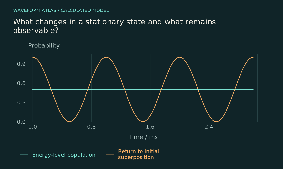
For projection back onto the initial equal superposition, the return probability is [1+cos(ΔEt/ℏ)]/2. If ΔE = h×1,000 hertz, the probability repeats every millisecond. This is an original two-level teaching example. It illustrates coherent beating, not decay: the probability falls and rises periodically, and no energy loss or fundamental reduction is required. A detector that samples only a falling portion could misidentify the process without a longer time scan.

Energy populations can remain fixed while other observables change

In that two-energy superposition, measuring energy gives E0 or E1 with equal probability at every time. The energy populations are stationary even though a complementary measurement oscillates. Thus the phrase the state is changing must be connected to the observable. One histogram can remain constant while another reveals coherent evolution.

The density matrix makes this transparent. Its diagonal entries in the energy basis remain one half, while its off-diagonal entries rotate with the relative phase. A measurement diagonal in that basis is insensitive to those entries. A measurement with off-diagonal components can detect them. This is the same reason that population measurements alone cannot establish all coherence properties of a state. Time-dependent phase information requires an appropriate reference and measurement basis.

Degeneracy changes the set of stationary vectors

If several orthogonal states share the same energy eigenvalue, any superposition within that degenerate eigenspace acquires the same global phase. It is therefore also stationary under the same time-independent Hamiltonian. The fact that a vector is written as a sum of basis states does not by itself imply time-dependent interference. The relevant question is whether the components have different energies under the Hamiltonian governing the evolution.

This observation prevents a misleading shortcut: counting terms in a state expression cannot determine whether a packet will change shape. A basis decomposition is a representation choice, while energy differences determine relative phase rates. Conversely, an apparently simple spatial profile can contain many energy components and evolve substantially. The correct diagnostic is the spectral content of the prepared state and the observable of interest, not the visual complexity of the notation.

Stationary density can coexist with current

A particle on a ring of circumference L offers a useful example. A normalized momentum eigenstate has wavefunction exp(ikx)/√L with k = 2πn/L. Its density is uniform and stationary. Yet its probability current is j = ℏk/(mL), which is nonzero for nonzero n. Stationary density therefore does not mean that every flow-related observable vanishes.

The example is normalizable because the ring has finite circumference. A free-space plane wave is often used for intuition but is not a normalizable localized state on an infinite line. Keeping this distinction explicit avoids treating an ideal momentum eigenfunction as a physically localized particle packet. A packet built from several allowed momenta can have a nonuniform profile and different evolution. The boundary conditions and preparation determine which model is appropriate.

A mixture can also be stationary

A density operator diagonal in the energy basis remains stationary under a time-independent Hamiltonian. More generally, the condition [ρ,H] = 0 gives no unitary change in ρ. A thermal equilibrium state of the form proportional to exp(−βH) satisfies this condition. Stationarity is therefore not restricted to pure energy eigenstates; mixed ensembles can also have time-independent statistics.

The converse needs care when discussing a limited set of measurements. A particular observable can remain constant even when [ρ,H] is nonzero. Establishing full stationarity requires more than one unchanging detector count. The state may have coherences invisible to that measurement. A practical claim should say whether the entire modeled density operator is stationary or whether only selected observables have been shown to remain constant over the tested interval.

A changing Hamiltonian can break stationarity

The energy-eigenstate result assumes the Hamiltonian remains fixed. If a field, boundary or coupling changes, the initial eigenstate may no longer be an eigenstate of the new Hamiltonian. Subsequent evolution can then produce transitions, shape changes or phase dynamics. The cause is the intervention encoded in H(t), not the bare passage of time.

Even a slow change requires an appropriate adiabatic analysis and assumptions about gaps and timescales. An abrupt change can populate several new energy components. A report should therefore state whether the apparatus parameters were held constant and how fluctuations were bounded. A state called stationary relative to one Hamiltonian is not guaranteed to remain so when the physical system is altered. The word describes a relation between preparation and dynamics.

Coupling to an environment changes the question

A subsystem initially in an eigenstate of its isolated Hamiltonian can relax or dephase when coupled to an environment. The isolated Hamiltonian no longer gives the complete dynamics. For example, an excited atomic state coupled to radiation modes can lose excitation even though it was an eigenstate of the simplified atom-only model. The combined interaction and available field states must be included.

This does not contradict stationary-state quantum mechanics. It shows that the chosen subsystem Hamiltonian omitted a relevant coupling. A true eigenstate of the full closed Hamiltonian would evolve by a global phase, but preparing and identifying such a state can be very different from preparing a nominal bare excitation. The distinction between an exact eigenstate and an approximate metastable preparation is central to understanding lifetimes and emission without treating time as an independent destructive agent.

Test stationarity with complementary observations

To assess a stationary-state claim, identify the Hamiltonian, verify the preparation and measure observables capable of revealing relevant coherences. A constant energy histogram alone does not exclude relative-phase evolution. A time scan in a complementary basis can reveal beating. A current measurement can distinguish a stationary density with flow from one without it. Environmental and control drift must be included in the uncertainty.

The lesson is that stationary is an exact statement within a defined model, not a synonym for inert or motionless. Global phase evolution can be present without changing probabilities; relative phases can produce oscillations without loss; and omitted couplings can make an apparently stationary subsystem evolve. These distinctions provide a precise way to decide what a time-dependent trace means and which physical assumption should be examined when the observed behavior differs from the ideal prediction.

The two-level example also supplies a simple frequency check. Adding the same constant C to both energies multiplies the whole state by exp(−iCt/ℏ), leaving every probability unchanged. The beating frequency depends only on E1−E0. If a calculation predicts a different interference period merely because the zero of energy was shifted, it has retained an unphysical global phase as though it were observable. This check is especially useful in numerical simulations, where large absolute energies can obscure a small relevant splitting. Removing a common phase can simplify the computation while preserving the measured dynamics, provided that relative phases and any explicitly time-dependent couplings are treated consistently.

Go to the original work.

These links identify the sources behind specific claims. Verification scope varies by source and is stated below.

1. 1 / University teachingMIT OpenCourseWare, Stationary states: key equations ↗

   MIT OpenCourseWare, Stationary states: key equations. https://ocw.mit.edu/courses/8-04-quantum-physics-i-spring-2016/resources/stationary-states-key-equations/

   Energy eigenstates and stationary probability densities.

   Verification scope: Official lesson record inspected; examples are explicitly defined teaching calculations.

2. 2 / University teachingPreskill, Quantum Information, Chapter 2: States and Ensembles ↗

   Preskill, J. Quantum Information, Chapter 2: States and Ensembles. Caltech lecture notes (2015 version).

   Density operators, composite states, measurement probabilities, quantum erasure and local statistics.

   Verification scope: Author-hosted lecture PDF inspected for relevant foundational definitions; independent elementary examples are worked in the article.

3. 3 / University teachingMIT OpenCourseWare, Quantum Physics I (2016), lecture notes ↗

   MIT OpenCourseWare, Quantum Physics I (2016), lecture notes. https://ocw.mit.edu/courses/8-04-quantum-physics-i-spring-2016/pages/lecture-notes/

   Schrödinger evolution, stationary states, Fourier wavepackets, observables and time delay.

   Verification scope: Official course notes index and named lesson records inspected; articles provide original elementary derivations.

4. 4 / University teachingPreskill, Quantum Information, Chapter 3: Measurement and Evolution ↗

   J. Preskill (2018). Lecture Notes for Ph219/CS219, Chapter 3: Foundations II: Measurement and Evolution, updated October 2018. Caltech.

   Measurement operators, channels, dephasing, amplitude damping and open-system evolution.

   Verification scope: Author-hosted PDF: §§3.4.2–3.4.3 dephasing and amplitude damping; §3.5.3 damped harmonic oscillator; §§3.6.1–3.6.2 Gaussian phase noise and spin echo. Relevant passages checked; no claim that this chapter treats detector timing or lifetime statistics.

5. 5 / University teaching8.044 Chapter 6: Statistical Mechanics at Fixed Temperature (Canonical Ensemble) ↗

   John McGreevy (2012). 8.044 Chapter 6: Statistical Mechanics at Fixed Temperature (Canonical Ensemble). https://mcgreevy.physics.ucsd.edu/s12/lecture-notes/chapter06.pdf

   Canonical Boltzmann weights; classical equipartition and quantum oscillator mean occupation.

   Verification scope: §6.1; §6.4 pp. 6-20–6-22; §6.5 pp. 6-23–6-26 inspected; numerical examples in the article remain independent calculations.

6. 6 / University teachingMIT: Entanglement, Density Matrices, and Decoherence ↗

   Aram W. Harrow (2016). 8.06 Chapter 3: Entanglement, Density Matrices, and Decoherence. MIT OpenCourseWare.

   Density operators and reduced states distinguish local observables from joint correlations.

   Verification scope: Official full chapter text inspected at §§1–4 for states, density operators and reduced dynamics, and §5.1 for interference and environmental records. Worked examples in this article are independent calculations.

7. 7 / University teaching8.04 Lecture Note 10 ↗

   Barton Zwiebach (2016). 8.04 Lecture Note 10. https://ocw.mit.edu/courses/8-04-quantum-physics-i-spring-2016/01b09433137651bedbbfe4f039b0c5be_MIT8_04S16_LecNotes10.pdf

   Stationary eigenstates, superpositions and a free particle on a circle.

   Verification scope: Stationary states and free particle on a circle inspected; numerical examples in the article remain independent calculations.

8. 8 / University teaching8.04 Lecture Note 6 ↗

   Barton Zwiebach (2016). 8.04 Lecture Note 6. https://ocw.mit.edu/courses/8-04-quantum-physics-i-spring-2016/d87c768c4e1181fde8d4366112169719_MIT8_04S16_LecNotes6.pdf

   Normalization, probability current and current conservation.

   Verification scope: Normalization and probability-current sections inspected; numerical examples in the article remain independent calculations.