Replacing 'time destroys it' with a measurable explanation

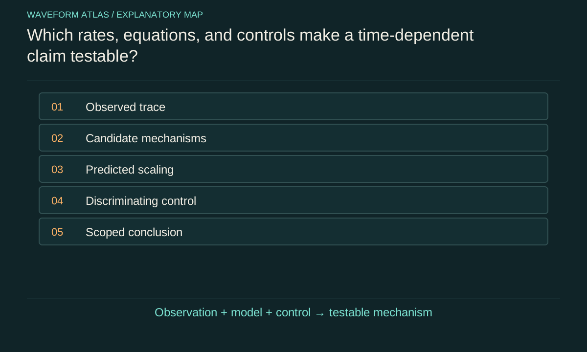
Translate the claim into an observable

The sentence time destroys the wave is too broad to test. Begin by asking what the instrument actually recorded. Was it a field amplitude, intensity, particle count, population, probability density, fringe contrast or correlation? These quantities can change differently. A lower local amplitude can reflect translation, a broader packet or energy loss. A reduced visibility can reflect dephasing, imbalance or reference drift. The first task is to name the measured quantity.

Write its units and normalization. A probability density is not a probability until integrated over a region. A count rate depends on source strength and detection efficiency. A normalized contrast can hide changes in total signal. This bookkeeping is not pedantry: it determines which conservation law or evolution equation is relevant. Without it, the same falling line can support several incompatible verbal explanations.

Define the initial condition and time origin

A time-dependent prediction begins from a specified preparation. State how the wave or quantum state was created, which degrees of freedom were controlled and what event defines t = 0. A preparation pulse with finite duration can broaden an apparent decay curve. A herald may select a different ensemble from the full source. An unrecorded phase can turn a coherent preparation into an ensemble average with reduced contrast.

The time origin should correspond to a physical record with known uncertainty. Synchronization offsets, cable delays and detector response can shift the trace. If different trials have different preparation times, the model should average over that distribution. A precise clock display does not guarantee a precise physical start. The preparation and timing uncertainty belong in the prediction before any residual is assigned to a new mechanism.

List mechanisms that predict the same first impression

A localized pulse can leave the detector window, disperse into a broader shape, transfer energy to matter or become correlated with an environment. Phase averaging can reduce an interference signal while individual runs remain coherent. A detector can lose sensitivity or saturate. Each process can make a selected trace smaller, but each predicts a different pattern under suitable additional measurements.

The list should be specific to the apparatus rather than an unlimited catalogue of possibilities. Identify the most plausible channels and calculate their expected dependence on distance, bandwidth, pressure, temperature, probe strength or duration. A good competing explanation makes a quantitative prediction. Simply naming decoherence or collapse without specifying the relevant coupling and observable does not resolve the ambiguity; it replaces one broad word with another.

Write the simplest adequate model

For a damped oscillator, an amplitude envelope might be A(t) = A0exp(−γt). For a constant-rate population, S(t) = exp(−Γt). For Gaussian phase dispersion, coherence might be exp(−σ²t²/2). For a freely spreading Gaussian packet, width grows as the square root of a quadratic function of time. These models are mathematically different even though each can lower a peak or signal over part of a trace.

Choose the model from the physical mechanism and test its adequacy. Do not select an exponential solely because a semilog plot looks approximately straight over a short interval. Several functions can fit a limited range. State which parameters are independently known and which are fitted. If every nuisance parameter is allowed to vary freely, the model may describe the data without identifying the cause.

Check amplitude and energy with one calculation

Suppose a calibrated oscillator amplitude falls to one half after ten milliseconds. Under A = A0exp(−γt), γ = ln2/0.010, about 69.3 per second. If stored energy is proportional to amplitude squared, the energy has fallen to one quarter and its exponential rate is 138.6 per second. The amplitude time constant is about 14.4 milliseconds, while the energy time constant is about 7.21 milliseconds.

These two constants describe the same ideal oscillator. Calling them contradictory lifetimes would confuse observables. Conversely, if measured energy does not follow the square of the amplitude under the expected conditions, the model or calibration needs attention. The example shows why an explicit equation can resolve a vague time claim before any foundational debate is needed. It also identifies an independent consistency check using two measured quantities.

Measure a conserved or complementary quantity

A complementary measurement can reveal where the missing signal went. If a packet broadens, integrate over a larger spatial region to test normalization or energy conservation. If a narrow-band signal weakens after modulation, inspect other frequencies. If a fringe fades, measure path populations and reference stability. If an excited population decays, look for emitted energy or other transition products within the detector’s acceptance.

The second observable should be chosen to distinguish the leading models. Measuring the same quantity with another color scheme adds little. A local amplitude and a total energy balance answer different questions; a population and a phase-sensitive correlation do too. The aim is to turn one ambiguous trace into a set of mutually constraining predictions. Agreement across those observables is stronger evidence than visual similarity to a familiar decay curve.

Use controlled interventions

Change a parameter that the candidate mechanism predicts should matter. Vary propagation distance to test delay, bandwidth to test dispersion, pressure to test collisions or probe strength to test measurement-induced dephasing. Interleave settings to reduce drift bias and monitor calibration throughout. The intervention should preserve other relevant conditions as well as the apparatus permits, with unavoidable correlated changes included in the model.

A useful control can also apply a recovery operation. Dispersion compensation or an echo may restore a signal if the relevant phase information remains accessible. Successful recovery constrains claims of irreversible destruction. Failure requires further diagnosis because imperfect control, energy loss and inaccessible environmental records can all prevent restoration. The control is informative only when its own fidelity and intended target are characterized.

Include the observation process in the fit

The measured trace can be a convolution of physical evolution with preparation and detector response. Finite windows, dead time, background and selection rules can reshape it. A constant background can flatten a tail; a threshold can shift an apparent arrival; missed early events can bias a fitted lifetime. These effects can mimic changes in the physical rate if they are omitted.

Fit a model for the recorded data rather than an ideal state variable disconnected from the detector. Preserve raw counts and timing records so that residual structure can be inspected. Report uncertainty from calibration and model choice as well as counting noise. A small formal fit error does not guarantee that the inferred mechanism is correct. The uncertainty should reflect the weakest important link in the preparation-to-record chain.

Define what would count against the preferred explanation

Before interpreting an anomaly, state a result that the proposed mechanism would not accommodate under its fixed assumptions. A gravity-related collapse model might predict a particular geometry dependence and accompanying heating; an ordinary loss model might predict energy transfer without phase-selective effects. If the observed pattern contradicts those requirements, the explanation should be revised or rejected. A mechanism that can be adjusted after every outcome is not being tested decisively.

A new-physics claim requires the conventional baseline to be constrained and the additional prediction to be explicit. The mere persistence of an unexplained residual is not a positive identification. Replication under changed conditions and an independent observable can make the inference stronger. Equally, a null result can be valuable when it excludes a specified parameter range rather than being described as nothing happening.

Write the conclusion as a scoped physical statement

Replace time destroyed the wave with a statement such as: the measured local energy decayed exponentially over the tested interval because it coupled to a calibrated loss channel, or the packet’s peak decreased while its integrated probability remained constant and its width followed free dispersion. If the mechanism remains uncertain, say which alternatives survived the controls. This preserves the result without inventing a cause.

The audit ends with a traceable chain: preparation, dynamics, observable, detector, comparison and uncertainty. Each link can be checked or improved. Time remains an essential experimental variable, but its role is to organize the evolution being measured. The physical explanation comes from the law and interaction that predict the change, and the evidence comes from controls that make competing explanations disagree.

A reference channel can help test whether a falling signal is an apparatus drift. If both a stable reference and the target are multiplied by the same time-dependent detection gain, their ratio can cancel that common factor. The cancellation is valid only if the channels share the relevant response and remain within the detector’s linear range. Different wavelengths, amplitudes or timing can invalidate the assumption. A ratio that remains stable is therefore a useful diagnostic, not an automatic proof that the target itself is unchanged. Compare absolute counts and the reference calibration as well. This example illustrates the audit’s general rule: every proposed correction is another physical model whose assumptions should be checked before its output is treated as a direct property of the wave.

Go to the original work.

These links identify the sources behind specific claims. Verification scope varies by source and is stated below.

1. 1 / University teachingPreskill, Quantum Information, Chapter 2: States and Ensembles ↗

   Density operators, composite states, measurement probabilities, quantum erasure and local statistics.

   Verification scope: Author-hosted lecture PDF inspected for relevant foundational definitions; independent elementary examples are worked in the article.

2. 2 / University teachingMIT OpenCourseWare, Quantum Physics I (2016), lecture notes ↗

   Schrödinger evolution, stationary states, Fourier wavepackets, observables and time delay.

   Verification scope: Official course notes index and named lesson records inspected; articles provide original elementary derivations.

3. 3 / University teachingPreskill, Quantum Information, Chapter 3: Measurement and Evolution ↗

   Measurement operators, channels, dephasing, amplitude damping and open-system evolution.

   Verification scope: Author-hosted lecture PDF inspected for relevant sections; not an exhaustive audit of every lecture derivation.

4. 4 / Primary theoryBassi et al., Models of Wave-function Collapse, Underlying Theories, and Experimental Tests ↗

   Research authors’ synthesis of stochastic collapse dynamics, motivation and distinct experimental signatures.

   Verification scope: Author-posted review abstract and bibliographic record inspected; general equations below are explicitly specified teaching models.