What does a coherence time measure?

Name the correlation before naming its time

Coherence describes phase relationships that can affect interference. A coherence time summarizes how a particular phase-sensitive quantity changes with delay. For a qubit, that quantity may be an off-diagonal density-matrix element in a chosen basis. For an optical field, it may be a first-order field correlation. For an interferometer, it may be a visibility envelope after accounting for balance and detector response. These definitions are related but not numerically interchangeable.

A report should therefore identify the preparation, correlation function, fitting form and measurement sequence. Saying that a system has a coherence time of one millisecond is incomplete without those details. Different degrees of freedom in the same apparatus can have very different coherence properties. Even the same degree of freedom can yield different times under free evolution, echo control and continuous driving because those protocols filter noise differently.

Separate phase memory from populations

For a two-level system, write a density matrix with populations on the diagonal and coherence off the diagonal. Pure dephasing can reduce the off-diagonal element while leaving the populations unchanged. The system may retain the same mean energy while losing a phase-sensitive signal. Energy relaxation changes populations and generally also affects coherence. The two processes are distinct even when one experiment is sensitive to both.

A concrete example begins with |+⟩. Complete dephasing in the zero/one basis produces an equal mixture, so a zero/one measurement remains fifty-fifty before and after. A plus/minus measurement changes from a definite plus result to equal probabilities. The lost signal is therefore a phase relation, not a disappearance of the two-level system or a necessary loss of its population. The chosen basis is part of this statement.

Define T1 and T2 in a simple model

In a standard Markovian two-level model, T1 describes exponential relaxation of a population difference toward equilibrium, while T2 describes exponential decay of transverse coherence. If an independent pure-dephasing contribution has time Tφ, the rates satisfy 1/T2 = 1/(2T1) + 1/Tφ. The factor of two reflects how population relaxation enters an off-diagonal amplitude. It is not an arbitrary convention that can be dropped without changing the model.

For T1 = 40 microseconds and Tφ = 80 microseconds, the two contributions are both 1/(80 microseconds), giving T2 = 40 microseconds. If pure dephasing vanishes, this model gives T2 = 2T1. The relation and bound apply under the stated assumptions. Non-Markovian dynamics, different definitions or complex multilevel fitting can require a different analysis, so they should not be treated as a universal identity for every quantity called coherence time.

The rate decomposition here combines the amplitude-damping coherence factor in Preskill §3.4.3 with the independent dephasing factor in §3.4.2: multiplying their exponentials adds their rates.

Static frequency spread can mimic decay

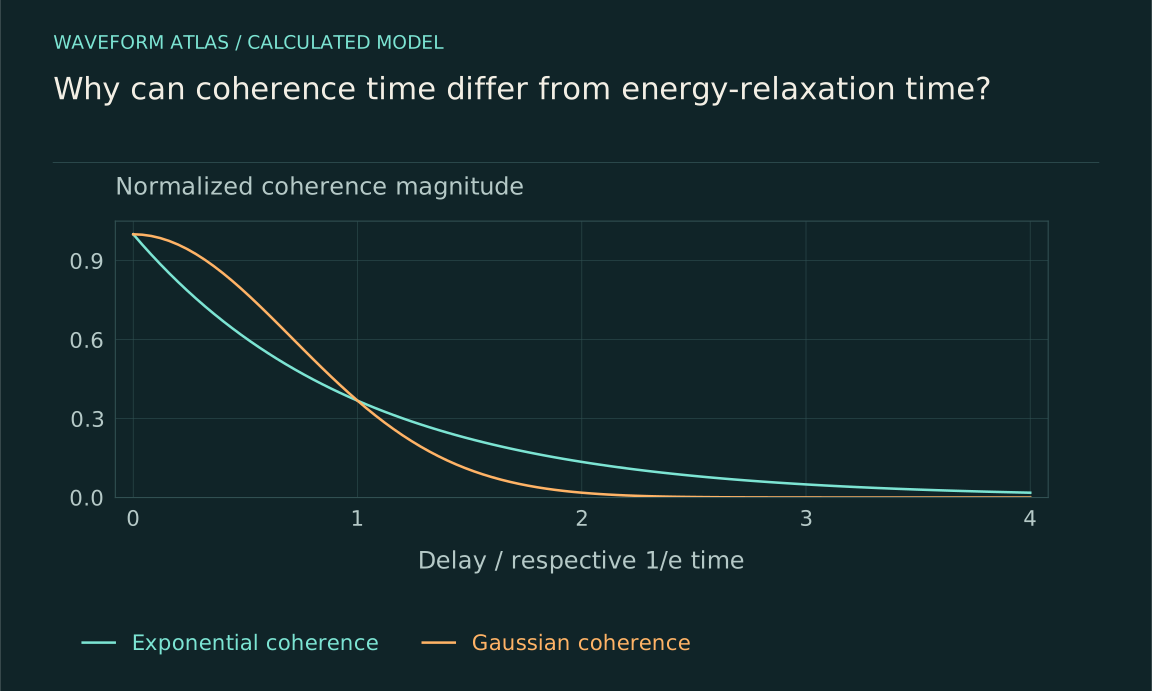
Suppose each member of an ensemble evolves coherently but has a slightly different frequency offset δω. Averaging their phases gives a coherence factor C(t) = ⟨exp(−iδωt)⟩. For a Gaussian distribution of offsets with standard deviation σω, this becomes exp(−σω²t²/2). The ensemble signal has a Gaussian envelope even though each member retains a definite phase relative to its own frequency.

If the coherence time is defined as the time when this envelope reaches 1/e, it is √2/σω. Another convention, such as an integral correlation time or half-height width, gives a different number. The fitting form and definition must accompany the value. This example also shows why an exponential fit can be misleading: a visually falling trace can arise from a distribution of coherent frequencies rather than a constant memoryless dephasing rate.

An echo can refocus some contributions

For a qubit with a static frequency offset during a trial, an ideal inversion pulse halfway through a sequence can reverse the accumulated relative phase in the toggling-frame description. The offsets then refocus at the echo time. This can restore an ensemble signal lost through inhomogeneous broadening. The recovered contrast demonstrates that the information was accessible to that control sequence under the tested conditions.

An echo does not reverse every source of decoherence. Rapidly fluctuating noise, energy relaxation, pulse errors and uncontrolled couplings can remain. The coherence time inferred from an echo therefore answers a different question from a free-induction time, often labeled T2*. Comparing them helps diagnose noise timescales, but a longer echo time is not evidence that the clock ran differently. The control changed how the system responded to its environment.

Optical coherence uses field correlations

For a stationary optical field, a normalized first-order correlation can be written g1(τ) = ⟨E*(t)E(t+τ)⟩ divided by the appropriate intensity normalization. Its magnitude determines interference between delayed copies under suitable conditions. A coherence time summarizes the delay range over which that correlation remains appreciable. It is not automatically the lifetime of an individual photon or the duration of every detected pulse.

Spectral width and temporal coherence are related through Fourier structure, but the numerical conversion depends on the spectral shape and convention. An exponential |g1| envelope corresponds to a Lorentzian-type line under standard assumptions; a Gaussian spectrum gives a Gaussian correlation envelope. Quoting a linewidth-to-time formula without specifying angular frequency versus ordinary frequency can also introduce factors of 2π. The units and shape should be written explicitly when numerical values matter.

These line-shape statements follow by Fourier transforming the specified correlation: exp(−|τ|/τc) gives a factor proportional to [1+(Δωτc)²]⁻¹, while a Gaussian transforms to another Gaussian. They are mathematical examples under the stationary-field assumption, rather than an additional result attributed to the quantum-mechanics course index.

Visibility is affected by more than coherence

An interferometer’s measured visibility can fall because of unequal path intensities, detector averaging, polarization mismatch or phase drift. Only after those effects are modeled can visibility be used as a direct estimate of a particular coherence function. For balanced ideal paths with a coherence factor c, visibility can equal |c|. With path probabilities p and 1−p, an additional factor 2√[p(1−p)] appears.

This matters in a delay scan because transmission or alignment may change with the delay setting. A lower fringe contrast at longer delay could then include a technical change unrelated to intrinsic phase memory. Measure path powers, detector response and reference stability alongside the fringes. A coherence-time fit should follow a model of the full measurement rather than assign every reduction in normalized contrast to one physical rate.

Measurement itself can influence coherence

Continuous monitoring or repeated readout can alter the dynamics being measured. A weak probe can introduce dephasing, heating or a conditioned trajectory even when each interaction is small. A strong measurement can reset the relevant state. The coherence time of an unmonitored system and the timescale observed under active measurement are therefore different operational quantities unless the probe’s effect is shown to be negligible or included in the model.

A useful control varies probe strength or duty cycle and extrapolates only within a justified physical model. If the fitted time changes strongly with readout power, the apparatus is participating in the process. That can be scientifically useful, but it should not be hidden under an intrinsic material parameter. The reported coherence belongs to the complete preparation, environment and interrogation protocol.

Fit the envelope without forcing a preferred mechanism

Inspect whether the data support an exponential, Gaussian, stretched or multi-component envelope before assigning a microscopic rate. Different forms can approximate the same short interval, so a limited fit range may not distinguish them. Background offsets and finite signal-to-noise can dominate the long-delay tail. The uncertainty in the fitted time should include these model choices when they materially affect the result.

A phase-resolved measurement can contain more information than an envelope alone. Frequency shifts, revivals or oscillatory residuals may reveal coherent coupling or nonstationary noise. Averaging them away can make a complicated process look like simple decay. Preserve the raw records and state the averaging procedure. A good coherence-time summary is a compact description of a tested model, not a replacement for the observable that was actually measured.

Use the time to choose a meaningful control

Once the relevant correlation and noise mechanism are identified, the time becomes useful for design. A short free-induction time caused by static offsets suggests refocusing or better homogeneity. A relaxation-limited T2 suggests reducing energy exchange. A readout-limited signal suggests changing the probe. These interventions target physical causes rather than trying to prevent time from passing.

The final account should state what phase relation was prepared, how it was interrogated, what envelope was fitted and which controls separated competing explanations. It should keep population lifetime, coherence time and detector integration time distinct. That precision explains why a system can retain energy after losing a fringe, why an echo can restore some signals and why different experiments can report different coherence times without contradicting one another.

For the Gaussian-offset example, take σω = 1,000 radians per second. At a delay of one millisecond, the ensemble coherence is exp(−1/2), about 0.607; its 1/e time is about 1.414 milliseconds. A static-offset echo can ideally restore that contribution even though the free-induction signal has fallen substantially. No population lifetime was specified, because this calculation does not require population relaxation. Adding an independent relaxation channel would multiply or otherwise modify the appropriate coherence evolution under the chosen model. Keeping these contributions separate lets an experiment predict what an echo should recover and what should remain lost. The result is a diagnosis of noise structure, rather than one universal number that claims to describe every way the system can change.

Go to the original work.

These links identify the sources behind specific claims. Verification scope varies by source and is stated below.

1. 1 / University teachingPreskill, Quantum Information, Chapter 3: Measurement and Evolution ↗

   J. Preskill (2018). Lecture Notes for Ph219/CS219, Chapter 3: Foundations II: Measurement and Evolution, updated October 2018. Caltech.

   Measurement operators, channels, dephasing, amplitude damping and open-system evolution.

   Verification scope: Author-hosted PDF: §§3.4.2–3.4.3 dephasing and amplitude damping; §3.5.3 damped harmonic oscillator; §§3.6.1–3.6.2 Gaussian phase noise and spin echo. Relevant passages checked; no claim that this chapter treats detector timing or lifetime statistics.

2. 2 / University teachingMIT OpenCourseWare, Quantum Physics I (2016), lecture notes ↗

   MIT OpenCourseWare, Quantum Physics I (2016), lecture notes. https://ocw.mit.edu/courses/8-04-quantum-physics-i-spring-2016/pages/lecture-notes/

   Schrödinger evolution, stationary states, Fourier wavepackets, observables and time delay.

   Verification scope: Official course notes index and named lesson records inspected; articles provide original elementary derivations.

3. 3 / University teachingPreskill, Quantum Information, Chapter 2: States and Ensembles ↗

   Preskill, J. Quantum Information, Chapter 2: States and Ensembles. Caltech lecture notes (2015 version).

   Density operators, composite states, measurement probabilities, quantum erasure and local statistics.

   Verification scope: Author-hosted lecture PDF inspected for relevant foundational definitions; independent elementary examples are worked in the article.

4. 4 / ReviewDecoherence, einselection, and the quantum origins of the classical ↗

   Wojciech H. Zurek. Reviews of Modern Physics 75, 715 (2003). Linked record is the author preprint.

   DOI: 10.1103/RevModPhys.75.715

   Environmental monitoring, preferred records and suppression of local interference.

   Verification scope: Publisher or author-institution abstract and bibliographic record inspected; full paper not audited.

5. 5 / University teachingECE 460 Lab 5: Interference and Temporal Coherence ↗

   University of Illinois Urbana-Champaign (2016). ECE 460 Lab 5: Interference and Temporal Coherence. https://light.ece.illinois.edu/ECE460/Labs2017/Lab%205%20Interference%20and%20Temporal%20Coherence.pdf

   First-order field correlation, interference visibility and the Fourier relation between optical spectrum and temporal coherence.

   Verification scope: p. 1, Background and Eqs. (1)–(2) inspected; numerical examples in the article remain independent calculations.

6. 6 / Primary theoryFringe Visibility and Which-Way Information: An Inequality ↗

   Berthold-Georg Englert. Physical Review Letters 77(11), 2154–2157 (1996).

   DOI: 10.1103/PhysRevLett.77.2154

   Visibility–distinguishability inequality; the equal-prior pure-record equality is derived explicitly in the article.

   Verification scope: Publisher or author-institution abstract and bibliographic record inspected; full paper not audited.