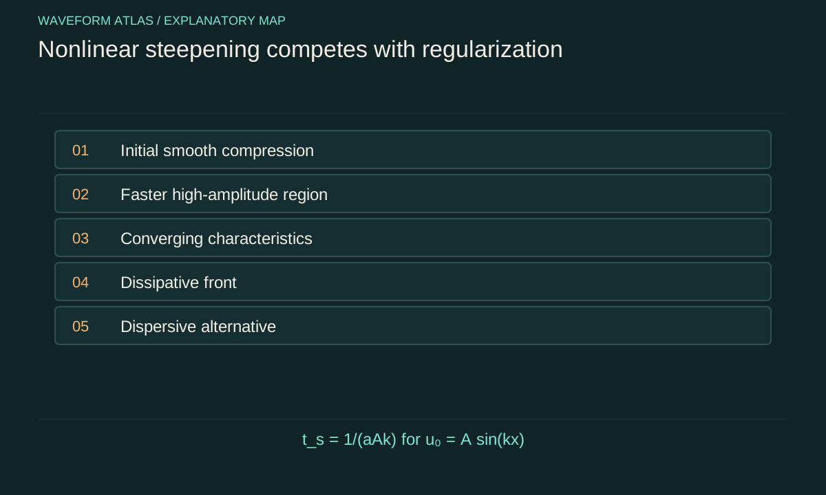
Sudden forcing and steep fronts

Sudden forcing and shock formation are different claims

An impact can launch a short pulse with a steep leading edge. Whether that pulse develops into a shock depends on the medium's nonlinear response, amplitude, propagation distance and dissipative or dispersive effects. A small acoustic pulse can remain well described by a linear wave equation even when its source acts briefly. Short duration alone does not establish a shock.

A shock is a thin transition between different flow or material states whose macroscopic description satisfies conservation jump conditions. Its internal thickness is set by physics beyond an ideal discontinuity model. In gases, viscosity and heat conduction regularize the front and entropy increases across a physical compressive shock. The visible edge is only one part of that definition.

Amplitude-dependent speed causes steepening

If a larger compressive disturbance travels faster than a smaller one ahead of it, characteristics converge and the profile steepens. A simple scalar illustration is u_t + a u u_x = 0. Each initial value moves at speed a u in this ideal equation. Regions with suitable negative slope develop increasingly large gradients as faster portions catch slower ones.

The scalar equation is an explanatory model, not a complete compressible-fluid description. It lacks the full thermodynamic state and dissipative structure of a gas shock. Its value is to isolate the kinematic mechanism of steepening. A physical prediction requires the actual equation of state, background flow and relevant transport coefficients.

Estimate the ideal steepening time

For the scalar model with initial profile u₀(x), the characteristic map is x = ξ + a u₀(ξ)t. Its derivative is 1 + a u₀′(ξ)t. The first zero marks gradient catastrophe in the inviscid model, giving t_s = −1/min[a u₀′] when that minimum is negative. The formula identifies both amplitude and length-scale dependence.

For u₀ = A sin(kx) with positive a, the minimum derivative is −aAk, so t_s = 1/(aAk). Doubling amplitude or wavenumber halves the ideal steepening time. These are original calculations within the scalar model. A real medium can disperse or dissipate the wave before this time, so the estimate is a comparison scale rather than a guaranteed shock-formation prediction.

Dissipation and dispersion regularize differently

Adding viscosity-like diffusion smooths steep gradients and can yield a shock layer of finite thickness. Adding dispersion can instead produce an oscillatory structure that spreads the steepening into a train of waves. The latter is often described as a dispersive shock in appropriate systems, but its microscopic energy and entropy account differs from a dissipative gas shock.

The distinction matters visually because both can follow a steepening event. A camera that resolves only the envelope may not distinguish a thin dissipative front from unresolved oscillations. Spectral and spatial measurements, together with the governing model, identify which regularization dominates. Do not infer irreversible heating solely from a steep edge if dispersive redistribution remains plausible.

Conservation supplies jump conditions

For a steady planar shock viewed in its rest frame, mass flux is continuous: ρ₁u₁ = ρ₂u₂. Momentum flux gives p₁ + ρ₁u₁² = p₂ + ρ₂u₂² in a simple inviscid outer-state description. Energy flux relates enthalpy and kinetic energy, with additional terms included when relevant. These equations connect the states on either side without resolving every detail inside the layer.

The NACA compressible-flow report provides an authoritative source for normal-shock relations in their specified assumptions. Applying those relations requires an appropriate gas model and upstream state. They should not be transplanted unchanged to water-wave breaking, a solid plastic front or an optical dispersive structure simply because each has a sharp transition.

The shock frame clarifies velocities

A front can move through the laboratory while fluid moves on either side. The velocities entering the jump equations are measured relative to the shock. Subtract the shock speed from laboratory velocities before using the steady shock-frame relations. Mixing frames can produce an apparent failure of mass or momentum conservation.

Measure front trajectory and upstream and downstream states on a common time base. If the front accelerates or curves strongly, a local approximation may be useful but should be stated. The front normal also determines the relevant velocity component. A projected image without geometric calibration may misestimate both speed and compression.

Compression and entropy distinguish physical branches

Conservation equations can admit mathematical discontinuities that are not physically realized under the stated conditions. An entropy condition selects the admissible compressive shock in ordinary gas dynamics. A rarefaction generally spreads as a continuous fan rather than behaving as the time reverse of a dissipative shock. Reversing a movie does not reverse the entropy production process.

This is another reason not to define a shock only by a jump in a plotted variable. The connection between states, propagation direction and thermodynamics matters. A measured density increase and pressure jump, combined with the correct frame and equation of state, provide stronger evidence than an isolated steep optical edge caused by illumination or image processing.

Weak and strong disturbances require different approximations

For small pressure and density variations, linear acoustics can describe propagation with nearly constant sound speed. As amplitude grows, nonlinear corrections can accumulate over distance. A wave can begin weak and steepen later, so the observation location matters. Conversely, a sharp initial pulse can decay or spread before developing a strong shock.

Compare nonlinear steepening length with attenuation and dispersion lengths. The shortest relevant scale often indicates which process dominates first. This scaling does not replace a full solution near competing regimes, but it guides an experiment and prevents universal claims that every impact necessarily generates a shock. The material response and propagation history determine the outcome.

Sensors must resolve the front without inventing it

A finite-bandwidth pressure sensor broadens a sharp front. A camera can blur it through exposure, while numerical differentiation can amplify noise and create artificial spikes. Calibrate temporal response and spatial resolution, and compare independent measurements when possible. The measured front thickness may be an instrument limit rather than a physical thickness.

Conversely, aggressive filtering or contrast enhancement can make a smooth variation look discontinuous. Retain raw data and document processing. To support a shock claim, estimate upstream and downstream states and front speed, then test the relevant jump relations within uncertainty. The combination is more robust than relying on a single processed image.

Account for the impact energy and later heating

The striker supplies energy that can enter compression, bulk flow, elastic waves and heat. A shock converts organized flow energy into internal energy while satisfying total energy conservation for the complete account. A detector that records only the outgoing coherent pulse can miss that conversion. The impact and medium must be treated together.

The accurate conclusion identifies the regime: linear pulse, nonlinear steepening, dissipative shock, dispersive front or a combination with other processes. It states the equation, measured states and resolution supporting that classification. Sudden forcing is the initiating event; shock formation is a particular dynamical outcome that requires its own evidence.

A normal-shock example tests the jump relations

For a calorically perfect ideal gas with heat-capacity ratio γ = 1.4 and upstream Mach number M₁ = 2 in the shock frame, the normal-shock density ratio is [(γ + 1)M₁²]/[(γ − 1)M₁² + 2]. Substitution gives 2.6667. The pressure ratio is 1 + [2γ/(γ + 1)](M₁² − 1), which gives 4.5. These are original calculations from the standard ideal-gas relations, not measurements of a particular impact.

The temperature ratio follows from the ideal-gas equation of state as the pressure ratio divided by the density ratio, giving 1.6875. Mass conservation then requires the downstream shock-frame speed to be three eighths of the upstream speed. The numbers provide several linked checks: density rises, speed falls in the shock frame and internal temperature increases while total energy flux is conserved under the stated assumptions.

Do not apply the example to a real gas outside the calorically perfect approximation without checking its thermodynamics. Strong heating can change heat capacities or activate additional processes. Curved, unsteady or oblique fronts also require the appropriate geometry and velocity components. The example is valuable because it shows what a quantitative shock claim entails, rather than because its chosen Mach number represents every sudden disturbance.

An experiment should measure enough upstream and downstream variables to test more than one relation. Fitting a pressure jump alone can leave density, speed and equation-of-state assumptions untested. Independent agreement across the linked quantities is much stronger evidence that the observed front belongs to the proposed shock regime.

A discontinuity in a numerical solution also needs a convergence check. Artificial numerical viscosity can broaden a front or change its apparent dissipation, while insufficient resolution can create oscillations. Compare conserved fluxes and resolved state jumps as the grid is refined. A visually sharp simulated line is not sufficient validation of a physical shock or its internal thickness.

A shock-frame velocity convention must accompany every numerical comparison of these ratios.

Go to the original work.

These links identify the sources behind specific claims. Verification scope varies by source and is stated below.

1. 1 / Official researchNACA Report 1135, Equations, Tables, and Charts for Compressible Flow ↗

   Mass, momentum and energy balance across compressible-flow shocks.

   Verification scope: NASA-hosted report record and normal-shock conservation passage inspected; illustrative scalar-wave models are kept separate.

2. 2 / University teachingMIT Physics III: Vibrations and Waves ↗

   Yen-Jie Lee. MIT Physics III: Vibrations and Waves. 2016.

   Wave equations, interfaces, optics and propagation in media.

   Verification scope: MIT course outline inspected; article derivations are independent textbook-level explanations.

3. 3 / University teachingOpenStax University Physics Volume 1: Impulse and Collisions ↗

   Impulse as the integral of force and the change of momentum.

   Verification scope: Open textbook section inspected; used for impulse as force integrated over time and change of momentum.

4. 4 / University teachingClass Meeting 24: Transport Equations and Burger’s Equation ↗

   J. Speck (2011). 18.152 Introduction to PDEs, Class Meeting 24: Transport Equations and Burger’s Equation. MIT OpenCourseWare.

   Inviscid Burgers characteristics and finite-time gradient singularities for a compressive initial slope.

   Verification scope: Sections 2–3 inspected, including constant values along characteristics and singularity formation. The atlas restores its coefficient a explicitly.