Build a phase-controlled interference demonstration

Choose a question the apparatus can answer

An interference demonstration should test a definite statement: two measured field contributions combine with a phase-dependent cross term at a specified detector. It should not begin by assuming that a low reading proves disappearance. A microphone can be disconnected, a beam can miss a photodiode, an amplifier can clip, and a software display can subtract an offset. Each produces darkness without demonstrating the intended mechanism.

A convenient acoustic version uses two speakers driven by coherent signals, a target microphone, and an independent reference channel. An optical version splits one source into two arms and recombines them while monitoring both output directions. The optical arrangement follows the logic of MIT's demonstration description, which explicitly considers where the light goes. Neither apparatus requires a claim about quantum collapse to make its measurements interesting.

Define the detector observable

For the acoustic version, record the microphone's complex response at a chosen tone frequency. Its amplitude and phase can be estimated relative to the electronic drive. Keep the microphone position fixed during the initial scan. Pressure is the relevant field variable; the square of its amplitude is a convenient signal metric, but interpreting it as directional acoustic intensity additionally requires information about particle velocity or an appropriate traveling-wave approximation.

For an optical photodiode, the ordinary time-averaged signal is proportional to received optical power within its calibrated operating range. It does not directly follow the rapid optical electric-field oscillation. The interference term survives because the two fields have a stable relative phase. State the detector area, bandwidth, averaging duration, and background subtraction method. Those choices define what spatial and temporal variation the recorded number includes.

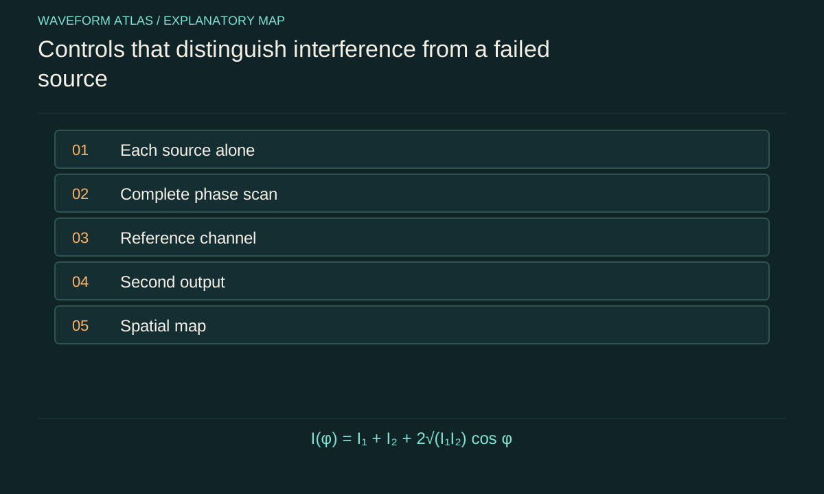
Check each contribution separately

Measure background with both sources blocked or disabled. Then measure source one alone and source two alone, with all downstream geometry unchanged. These runs establish individual signal levels and help identify unequal amplitudes. In an optical two-arm interferometer, blocking an arm is usually preferable to changing the source itself because changing source operation can also change its spectrum, pointing, or output power.

Call the background-corrected individual intensities I₁ and I₂. For fully overlapping coherent fields, the predicted combined intensity is I(φ)=I₁+I₂+2√(I₁I₂)cosφ. If the signal calibration uses arbitrary detector units, the same formula applies when those units are linear in intensity and share a common scale. A nonlinear display, automatic gain control, or saturating detector invalidates that simple comparison unless explicitly corrected.

Scan through the whole cycle

Vary relative phase through at least one complete cycle, sampling densely enough to resolve the minimum and maximum. A full scan is more diagnostic than tuning until one low reading appears. Fit an offset plus sinusoid and compare the fitted amplitude with the independently measured source contributions. A repeatable sinusoidal dependence identifies the cross term expected from coherent superposition under the stated single-frequency model.

As a calculated example, let I₁=1 and I₂=0.64 in common units. Perfect mode overlap predicts Imax=3.24 and Imin=0.04. A nonzero minimum in this case is expected from amplitude mismatch alone. Claiming that every nonzero residual disproves interference would be wrong. Conversely, a residual lower than the prediction may signal a change in source powers, an incorrect background correction, or an unmodeled detector response.

Use contrast to diagnose overlap

Define visibility V=(Imax−Imin)/(Imax+Imin). The example above gives V≈0.976. If the measured visibility is substantially lower while the individual intensities remain stable, consider polarization mismatch, spatial overlap, phase drift during averaging, or spectral bandwidth. Representing all these effects by an effective coherence factor can summarize the scan, but that one number does not uniquely identify the cause.

Change one suspected factor at a time. Rotate polarization in an optical apparatus, shorten the path imbalance, reduce vibration, or narrow the measurement bandwidth. If visibility changes in the predicted direction, the control supplies evidence about the limiting mechanism. The MIT demonstration index identifies several such controls. The teaching value comes from linking an intervention to a measured change, not from fitting every imperfection into an unexplained efficiency factor.

Keep a reference channel running

A reference monitor distinguishes a phase-driven minimum from a fading source. Record source power or drive amplitude throughout the phase scan and repeat the single-source checks afterward. Normalize cautiously: dividing by a noisy reference can introduce its own bias. The raw signals and the normalized result should both remain available for diagnosing drift, clipping, and unexpected correlations.

In the acoustic experiment, two speakers driven from one generator share a clock, which helps stabilize their frequency difference. Their actual acoustic phases still depend on electronics, speaker mechanics, and propagation. A reference electrical waveform therefore does not by itself prove equal pressure at the microphone. Measure the complete source-to-detector response. Likewise, equal optical arm lengths on a ruler do not guarantee equal phase when materials, polarization, or temperature differ.

Look beyond the dark point

Move the acoustic microphone along a recorded path after establishing the phase setting at the target. Map where cancellation weakens and where reinforcement appears. Keep the source geometry fixed and note any effect of the microphone stand or nearby reflecting objects. A spatial map demonstrates that the control condition is local and helps explain why a quiet point does not imply a quiet room.

For the optical version, monitor both interferometer outputs simultaneously. In an ideal balanced lossless arrangement, their powers vary complementarily as phase changes. Their sum stays constant if input power stays constant. Real data can include losses and unequal detector efficiencies, so calibrate each channel before comparing sums. A complementary trend is strong evidence for routing between outputs; a constant sum without calibration is only suggestive.

Separate a floor from a zero

Every detector has finite sensitivity, background fluctuations, and a range over which its response is linear. If the minimum is indistinguishable from the background, report an upper bound based on the measurement uncertainty. Do not replace that bound with an exact zero. Repeating measurements estimates random variability, while calibration checks address systematic errors that repeated sampling alone cannot remove.

A phase scan also needs uncertainty in its horizontal coordinate. Mechanical drift or an imprecise actuator can blur the apparent notch. Near a perfect equal-amplitude minimum, the residual scales quadratically with small phase error. That makes the minimum very sensitive to jitter even when the rest of the sinusoid looks clean. Recording a time series at the minimum helps distinguish a stable small residual from rapid excursions averaged into one number.

Finite sampling also changes the uncertainty of a measured contrast. Suppose independent intensity measurements near a bright maximum have standard uncertainty 0.01 in normalized units, while the minimum is 0.02 with comparable uncertainty. The minimum is then poorly resolved relative to its own size even though the maximum may be known precisely. Reporting many decimal places in visibility would conceal that limitation. Propagate uncertainties through the contrast formula or use repeated complete scans to estimate the spread of fitted contrast.

Randomize or alternate phase settings when slow source drift is plausible. A scan that always moves from maximum to minimum can confuse a steadily decreasing source with a deeper fringe. Interleaving reference phases makes that drift visible. Preserve the order and timing of measurements so that such effects can be checked afterward. These steps concern inference from the data, not an extra physical cancellation mechanism; they make the claimed depth of suppression credible.

Try a deliberate failure of the conditions

A useful demonstration includes controlled loss of cancellation. Slightly change one amplitude, introduce a delay, rotate one polarization, or move one source. Predict the direction and approximate magnitude of the residual before making the change. This makes the experiment a test of a model rather than a display assembled to produce a striking visual result.

For instance, equal unit field amplitudes at opposite phase cancel ideally. Reducing one amplitude to 0.9 leaves a residual field of 0.1 and an intensity of 0.01 in the same normalization. The maximum intensity becomes 3.61. This asymmetry between field error and intensity residual provides a quantitative check. Return the control to its original setting afterward: reproducible recovery helps distinguish a reversible phase condition from an accidental alignment change or source failure.

What to include in the result

A complete report gives the setup, detector observable, individual-source signals, phase scan, fitted model, uncertainties, and reference stability. It then shows either a second-output power measurement or a spatial map appropriate to the claimed conclusion. Raw or minimally processed traces make it possible to see whether averaging and background subtraction materially affect the interpretation.

The strongest modest conclusion is that the observed fields obey the predicted coherent-superposition relationship within stated uncertainty. A separate energy-flow claim requires the corresponding power measurements. A quantum claim requires suitable state preparation and quantum-sensitive observables. Keeping those levels explicit does not weaken the demonstration; it makes each result independently understandable and prevents a dramatic minimum from being asked to establish more physics than the apparatus measured.

Go to the original work.

These links identify the sources behind specific claims. Verification scope varies by source and is stated below.

1. 1 / University teachingMIT: Destructive Interference — Where Does the Light Go? ↗

   An interferometer demonstration follows light into both output directions.

   Verification scope: Official demonstration description inspected; no invented transcript quotation or timestamp.

2. 2 / University teachingMIT: Demonstrations in physical optics ↗

   MIT: Demonstrations in physical optics. https://ocw.mit.edu/courses/res-6-006-video-demonstrations-in-lasers-and-optics-spring-2008/pages/demonstrations-in-physical-optics/

   Demonstrations identify amplitude, polarization, vibration, path difference and spectrum as controls on fringe contrast.

   Verification scope: Official course demonstration index and descriptions inspected.