Evaluating claims of complete wave elimination

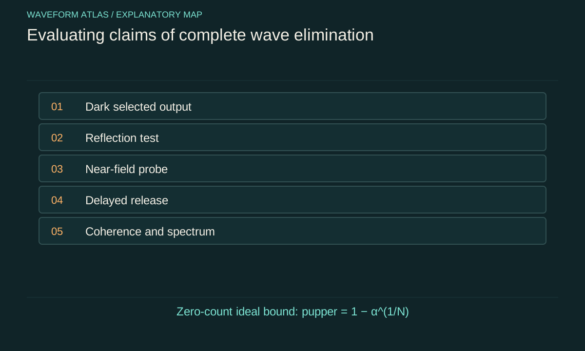
Define what complete elimination would mean

The phrase can refer to zero transmitted power, no detectable local field, no retained excitation, absorption of incoming photons or a proposed collapse of a superposition. These are not equivalent. A barrier can produce one while failing another. Write the claimed observable and system boundary before deciding which experiment tests it. An unrestricted statement about every field everywhere is much stronger than a measurement in one finite channel.

Also define the observation interval and frequency range. A pulse can be delayed or shifted outside the receiver band. Stored energy can emerge later. A local field may lie below spatial or temporal resolution. The conclusion should match those limits rather than treating an instrument's null reading as a mathematical proof about all unmeasured degrees of freedom.

Begin with the receiver's actual measurement

A receiver selects some combination of position, direction, polarization, frequency and spatial mode. A transformation that moves the wave outside that selection can make the output dark without removing the wave. Expand the aperture, scan alignment or use complementary mode detection to test that possibility. Keep the source independently monitored so that a weak input cannot masquerade as strong blocking.

Check detector linearity, bandwidth, background and processing. An automatic offset subtraction can create a zero mean, while a threshold can discard weak counts. An apparently exact zero in rounded software output may mean only below display resolution. Preserve raw data and calibration. The first scientific statement is about what that measurement chain can exclude, not about a mechanism inferred from its appearance.

Measure reflection as an explicit alternative

A nearly lossless barrier can return incident energy toward the source. The transmitted detector then reads little while the reflected channel carries most of the power. Measure that channel with a method that separates incident and reflected waves. Standing-wave interference near the source can otherwise complicate the interpretation of local amplitude.

Include source loading and all accessible directions. A reflected wave can change the generator's delivered power, so comparing only nominal settings can give an inconsistent budget. If reflection accounts for the missing transmission within uncertainty, the supported explanation is scattering into the return channel. That observation does not establish absorption or destruction of the complete field.

Look for evanescent penetration

Below cutoff or under total internal reflection, a field can remain near the boundary while decaying spatially. A suitable probe can detect it, although the probe itself can alter the coupling. The existence of that field directly distinguishes blocked travelling propagation from an empty region. State the direction of decay and the field component being measured.

A local evanescent field need not carry average power into a semi-infinite lossless forbidden direction. It can still store energy or couple to a nearby allowed channel. Adding a second structure can therefore change transmission without violating the original cutoff condition. A claim of complete elimination must consider these boundary-dependent possibilities rather than equating an imaginary longitudinal wave number with zero field.

Check delayed release and stored excitation

A cavity, defect or bound mode can retain an excitation while direct transmission is weak. After the input stops, a controlled release or ringdown measurement can reveal stored energy. In a quantum model, a stationary bound-state density with exponential tails is not a temporal disappearance process. The state remains normalized under its specified closed Hamiltonian.

A real stored excitation can decay through leakage or absorption, so measure lifetime separately from localization. A short observation window may miss a long-lived mode. Conversely, later output can originate in energy stored before the chosen input window. Include preparation and reset stages when testing a global elimination or energy-balance claim.

Absorption changes the material state

If incident light is absorbed, energy is transferred to matter and may subsequently become heat or other excitations. The photon population in the selected optical mode can decrease, but the complete energy account continues through the material. This ordinary process differs from asserting that energy vanished or that a universal objective-collapse mechanism was demonstrated.

Measure heating or other material responses where they can resolve the mechanism, and separate them from scattering into uncollected modes. For particles other than photons, the available absorption, capture or reaction channels depend on the system. Do not use the word annihilation as a generic synonym for attenuation. A claim about a specific particle reaction requires the corresponding products and conservation accounting.

A changing structure can move the frequency

Time-dependent boundaries or media can exchange energy with the controller and create sidebands. A detector tuned only to the original carrier can become dark even while significant output appears elsewhere in frequency. Measure the spectrum broadly enough to test that alternative and include the drive's energy contribution. Static scattering formulas are insufficient for a rapidly switched device.

The same principle applies to temporal filtering and pulse reshaping. A delayed or broadened signal may fall outside a fixed acquisition gate. Vary the time window and use an independently timed reference. The absence of counts in one gate is a statement about that gate, not proof that the entire prepared excitation ceased to exist.

Test coherence separately from survival

A reflected or transmitted amplitude can remain coherent with another reference even when its magnitude is small. Conversely, a surviving population can lose accessible phase relations through environmental coupling or technical noise. Measure both survival and a phase-sensitive observable if the claim concerns quantum state reduction. Neither quantity is a universal proxy for the other.

A complete lossless scattering transformation can be unitary across all outputs, while a selected output is described conditionally after discarding other events. Report that conditioning and its probability. A normalized survivor histogram cannot show that all initial probability remained. The experiment must distinguish a controlled redistribution, a measurement record and an added objective-reduction hypothesis rather than calling each one blocking.

Put a statistical bound on a null result

Suppose an ideal counting experiment has N independent incident trials, perfect detection of the selected transmitted outcome and zero observed transmissions. A one-sided upper bound at confidence level 1−α is p_upper=1−α^(1/N) under the binomial model. For N=1000 and α=0.05, it is approximately 0.00299. This is an illustrative calculation, not data from a performed experiment.

Finite efficiency, background and uncertain incident counts require a modified analysis. Zero observed events do not prove probability exactly zero. The bound states what transmission values are inconsistent with the null at the chosen statistical criterion and assumptions. Reporting it is more informative than declaring absolute elimination, because it makes the experiment's sensitivity and possible future improvement explicit.

For the stated zero-count case, the binomial probability is P(0|p)=(1−p)^N. Solving P(0|p_upper)=α yields the displayed exact bound; replacing p by ηp gives the efficiency correction below.

Require a distinct prediction from a new mechanism

A proposed new elimination or collapse model should specify how its effect depends on controlled variables and what it predicts beyond ordinary reflection, absorption and decoherence. It must preserve or explicitly modify the relevant conservation and probability laws in a consistent account. A dark detector is not a unique prediction if many established mechanisms produce the same result.

Choose measurements that separate those predictions: complementary ports, near fields, heating, delayed release, output spectrum or phase-sensitive recovery. Shared parameters should predict several conditions rather than being adjusted independently after every run. If an anomaly remains, reproduce it with independent calibration or a different readout. A discrepancy is a reason for investigation, not an automatic identification of the most dramatic explanation.

A rigorous report can establish a transmission upper bound for a named mode, near-total reflection, significant absorption, a trapped excitation or a specific loss of accessible coherence. It gives the geometry, timing, detector response and remaining unmeasured channels. It labels calculated diagrams and proposed tests separately from actual observations. These narrower conclusions can still represent substantial physical control.

Complete wave elimination is therefore a claim to be unpacked rather than assumed from darkness. Following energy, probability and phase through the full apparatus reveals whether propagation was blocked, the field was redirected, or an excitation changed form. That account supplies a concrete scientific result and identifies exactly what additional evidence would be needed for a stronger claim.

An efficiency correction shows how strongly a null depends on measurement assumptions. If each transmitted event is detected independently with known efficiency η and there is no background, the observed success probability is ηp. The zero-count bound therefore constrains p to [1−α^(1/N)]/η, capped at one. With N=1000, α=0.05 and η=0.5, the illustrative upper bound is about 0.00598, twice the perfect-detector value. Uncertainty in η must also be propagated. This calculation does not account for correlated trials, unknown backgrounds or an uncertain number of incident events; those require a more complete model. Stating such assumptions makes a strong suppression result reproducible without pretending that finite counting can demonstrate an exact universal absence.

If trials share a drifting source or correlated preparation error, the independence assumption can fail. Analyse the relevant blocks or an explicit correlated model before quoting a simple binomial bound.

Go to the original work.

These links identify the sources behind specific claims. Verification scope varies by source and is stated below.

1. 1 / University teachingHaus and Melcher, Electromagnetic Fields and Energy, Chapter 11: Energy, Power Flow, and Forces ↗

   Conservation of field energy including surface flux, stored energy, dissipation and electromechanical exchange.

   Verification scope: Official textbook chapter opening and integral energy-conservation section inspected; not a claim of reading all 90 pages.

2. 2 / University teachingMIT 6.013 (Spring 2009), L16: TEₘₙ rectangular waveguide, cavity resonators, perturbations ↗

   D. Staelin, MIT 6.013 Electromagnetics and Applications, Lecture 16: TEₘₙ rectangular waveguide, cavity resonators, perturbations (Spring 2009).

   TE/TM rectangular-guide dispersion and geometric cutoff under ideal assumptions.

   Verification scope: Official course index title and current download URL verified; PDF slides 3–6 read for dispersion, evanescence, mode restrictions and cavity frequencies.

3. 3 / University teachingMIT Quantum Physics II, Bound-state lecture transcript ↗

   Bound-state solutions decay at spatial infinity and satisfy quantized matching conditions.

   Verification scope: Official transcript excerpt on decaying tails and bound-state conditions inspected through search.

4. 4 / ReviewHornberger, Introduction to decoherence theory ↗

   K. Hornberger, Introduction to Decoherence Theory, in Entanglement and Decoherence, Lecture Notes in Physics 768, 221–276 (2009). Author manuscript: arXiv:quant-ph/0612118.

   DOI: 10.1007/978-3-540-88169-8_5

   Section 5.1: reduced density matrices, environmental-state overlaps and distinctions between decoherence and phase averaging.

   Verification scope: Targeted sections 5.1.1–5.1.4 and Eqs. (5.5)–(5.7) read in the author preprint; entire 57-page chapter not read.

5. 5 / University teachingZwiebach, MIT 8.06 Chapter 6: Adiabatic Approximation ↗

   B. Zwiebach, MIT 8.06 Quantum Physics III, Chapter 6: Adiabatic Approximation (Spring 2018 course; notes dated 2017).

   Time-dependent Hamiltonians, isolated-level adiabatic following, gap and coupling conditions, and Landau–Zener limitations; §1 also gives the classical oscillator action.

   Verification scope: Sections 1–3 and the Landau–Zener discussion inspected; not asserted as a general theorem for open scattering continua.