A longer wavelength is not a wider wavepacket

Two rulers on the same drawing

Imagine a short train of ripples enclosed by a smooth outline. A small ruler measures crest-to-crest spacing. A larger ruler measures the distance over which the ripple train is appreciable. Those rulers answer different questions. The first estimates the carrier wavelength. The second estimates the envelope width. A photograph can show both, but it cannot make them identical. This distinction is especially important when a drawing is stretched on a screen: the display transformation may change every length, while the proposed physical operation changes only one.

A carrier–envelope description is most useful when several oscillations fit under an envelope and the envelope varies relatively slowly. Very short or strongly distorted packets may have no single representative carrier. Even then, a spectrum and a properly defined spatial width remain useful. The failure of a convenient decomposition is a reason to use a fuller description, not a reason to assign every visible feature to one wavelength. State the convention before comparing measurements taken by different instruments or numerical programs.

Write the independent controls explicitly

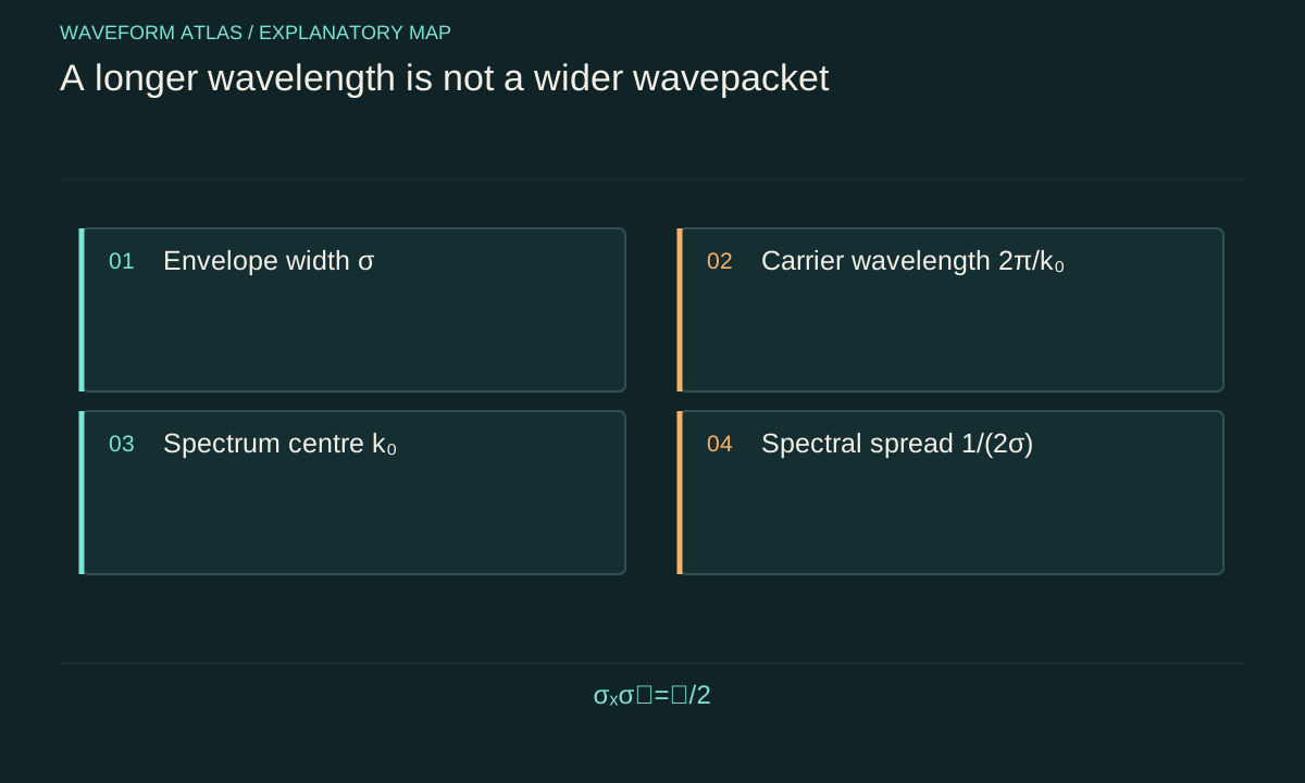
Use the complex model ψ(x)=N exp[−x²/(4σ²)] exp(ik₀x). Its probability density is a Gaussian with standard deviation σ. The carrier phase changes by one full turn over the distance 2π/k₀. Increasing σ widens the probability distribution. Increasing k₀ shortens the phase wavelength. These parameters appear in different factors, so their independence is visible before any Fourier transform is calculated.

The real part of ψ oscillates beneath the envelope, but |ψ|² does not show those carrier oscillations in this single-packet model. That difference matters when comparing a quantum probability image with a classical displacement trace. A camera recording optical intensity also usually averages over the rapid optical cycle. It measures a quantity related to field magnitude squared, not a movie of the carrier electric field. An absent visible carrier is therefore not evidence that the field has been flattened. It may simply reflect what the detector is designed to measure.

The spectrum has a centre and a width

Fourier transformation exchanges the spatial representation for a wave-number representation. For the Gaussian above, the momentum-space density is centred at ℏk₀. Its standard deviation is ℏ/(2σ). The central value and the spread are again separate properties. Shifting the entire spectrum changes the mean momentum. Narrowing that spectrum changes the spatial extent of the packet. A laboratory operation can do either, both, or something more complicated.

Consider two dimensionless states with σ=1 and carrier wave numbers k₀=4 and k₀=8. Their probability envelopes and momentum spreads are equal, but their mean momenta differ. Now compare σ=1 and σ=2 at fixed k₀=4. Their mean momenta match while the latter has half the momentum spread. These examples are calculated model comparisons, not experimental data. They demonstrate how to construct a test that changes one property at a time. They also show why a broad frequency spectrum does not mean that every component has a high frequency.

A translation does not broaden the packet

A shift in position adds another independent control. Replacing ψ(x) with ψ(x−x₀) moves the packet centre without changing its width. In wave-number space it introduces a phase factor. A momentum kick, by contrast, multiplies the position wavefunction by exp(iqx), shifting the momentum distribution without changing the instantaneous position density. These two operations can look deceptively quiet in one representation while being obvious in the other.

This provides a practical diagnostic. If an actuator changes a packet's later arrival position but leaves its immediate width unchanged, it may have delivered a momentum kick rather than a spatial dilation. If the apparatus moves the source or coordinate origin, it may produce a translation. Before fitting a width, subtract a fitted centre and report the centre separately. Otherwise, an ensemble of otherwise identical packets with fluctuating centres can appear broader when averaged. The resulting width combines intrinsic packet extent with preparation jitter, and those contributions should not be interpreted as the same physical process.

Dispersion links spectrum to later shape

A spectrum becomes a time-dependent waveform after each component accumulates the phase prescribed by its dispersion relation ω(k). Near a chosen centre k₀, the first derivative dω/dk gives the group velocity in a narrow-band approximation. Curvature d²ω/dk² causes different nearby components to acquire different relative phases and can alter the envelope. An initial width alone is therefore insufficient to predict a later width unless the medium and propagation law are known.

For a perfectly nondispersive model with ω=vk, all Fourier components translate together and the envelope keeps its shape. For a free nonrelativistic quantum particle, ω=ℏk²/(2m), so the curvature is nonzero and a typical localized packet spreads. The same initial drawing can consequently have different futures in different systems. This is the reason a visualization needs its governing equation displayed beside the sliders. An attractive animation without a dispersion law may illustrate a shape transformation, but it cannot establish that a physical device performs that transformation.

Width definitions can create false disagreements

A Gaussian amplitude width, a Gaussian intensity width, a root-mean-square width and a full width at half maximum are not interchangeable numbers. If an intensity distribution is proportional to exp[−x²/(2σ²)], its full width at half maximum is 2√(2 ln 2)σ, approximately 2.355σ. The amplitude has a different half-maximum width because it is the square root of the intensity. Comparing those widths without conversion creates an apparent change even when the underlying field is identical.

Choose a definition suited to the measurement. A full-width measure is intuitive for a single smooth peak but can become ambiguous for multiple peaks. A second moment includes tails and is sensitive to background subtraction. An encircled-power radius is useful for finite optical beams. A detector with a limited field of view can clip broad tails and bias all three. Report the raw profile, the fitting window and the background model when claiming a physical width change. The uncertainty in the width estimate belongs in the comparison, rather than being hidden behind a smooth fitted curve.

Measure phase as well as brightness

Two pulses can have the same spectral intensity and different temporal widths because their spectral phases differ. A chirped pulse is a familiar case: different frequency components reach the pulse maximum at different times. Removing the appropriate phase variation can shorten the pulse while preserving its spectral intensity in an ideal lossless model. Conversely, an intensity image by itself cannot reveal every phase distortion that will affect later propagation.

A useful measurement set therefore contains at least one phase-sensitive observable. In optics this might be interference with a known reference or an appropriate pulse-characterization method. In matter-wave experiments it may be controlled recombination and a phase scan. The exact apparatus depends on the system, but the logic is general. Do not infer a unique complex field from one magnitude-squared image when multiple fields could produce that image. The inverse problem needs enough information to distinguish those candidates. A model should make clear which phase information was measured and which was assumed during reconstruction.

Use independent sliders as an experimental rehearsal

An educational model should let the reader vary σ and k₀ independently, display the resulting envelope and phase oscillations, and show the matching spectrum. It should also expose normalization. If σ increases while total probability or total pulse energy is held fixed, the peak changes for a defined reason. If the peak is held fixed instead, the integrated quantity changes. Those are alternative experimental constraints, not cosmetic plotting options.

A useful next comparison freezes the initial spectrum and changes only the propagation law. Another freezes the medium and changes only the spectral phase. These controlled variations train the reader to ask which knob exists in a real apparatus. They also identify the measurements needed to validate a proposed stretcher or compressor. The central question is not whether a trace looks wider. It is whether the measured centre, width, phase, normalization and propagation agree with one specific mechanism. That richer description makes the distinction between wavelength and packet size experimentally useful.

As a practical width-conversion exercise, an intensity Gaussian with σ=2 millimetres has a full width at half maximum of about 4.710 millimetres. Its amplitude reaches half its peak farther from the centre because taking a square root changes the exponent. A report should therefore label a quoted width as amplitude, intensity or probability-density width. When software packages use different conventions, convert their parameters before comparing the plotted curves. This small bookkeeping step can prevent an apparent factor-of-√2 disagreement from being mistaken for a physical effect or an unexpected failure of the Fourier relation.

Go to the original work.

These links identify the sources behind specific claims. Verification scope varies by source and is stated below.

1. 1 / University teachingZwiebach, Quantum Physics I, Lecture 7: Wavepackets and uncertainty ↗

   Barton Zwiebach (2016). 8.04 Lecture Note 7. https://ocw.mit.edu/courses/8-04-quantum-physics-i-spring-2016/6ca5bd79a2121967796f7c0b8f6f48c9_MIT8_04S16_LecNotes7.pdf

   Fourier representation and unitary free-particle spreading; equations are used as standard fundamentals, with original worked examples.

   Verification scope: MIT lecture PDF text inspected; not a claim of experimental evidence.