Why a free quantum wavepacket spreads

Begin with a localized preparation

A free wavepacket is a model of a particle whose state is initially localized but is subsequently evolved without a potential. Localization does not require a single momentum. In fact, a finite position spread implies a momentum spread. The preparation might have used a trap, a source aperture or another controlled process, but the free-evolution model begins after that preparation has ended. It assumes that interactions and environmental disturbances can be neglected over the interval being studied.

This starting point should be stated explicitly. A packet released from an interacting gas, a charged particle near a surface, or an optical pulse in a nonlinear medium may not follow the simplest free law. Calling its later motion free is an approximation to check. The model is still valuable because it supplies a baseline with a definite prediction. If the data differ, the discrepancy directs attention toward the omitted forces, correlations, interactions or detector response. It does not automatically identify an unfamiliar mechanism.

Every momentum component advances its own phase

For a nonrelativistic particle of mass m, a momentum p has kinetic energy p²/(2m). During time t, the corresponding amplitude acquires the phase exp[−ip²t/(2mℏ)]. The magnitude of each momentum amplitude remains fixed. Returning to position space requires adding those components with their updated phases. Their changing interference pattern produces the evolving spatial distribution.

This is a useful way to understand spreading without picturing a probability fluid being pulled apart by an outside hand. There is no external stretching force in the model. Instead, the initial state contains components associated with different velocities, and quantum phase evolution organizes their contributions. The mean packet centre travels according to its mean momentum. The width describes how the distribution extends around that moving centre. Those two changes should be plotted separately, particularly when a detector samples the distribution at different flight times rather than photographing it continuously.

Derive the width from operator evolution

The free Heisenberg equations give x(t)=x(0)+p(0)t/m and p(t)=p(0). Squaring the centred position operator and taking its expectation yields a general variance relation: σₓ²(t)=σₓ²(0)+(2t/m)Cov(x,p)+(t²/m²)σₚ²(0). The covariance is the symmetrized expectation of the position and momentum fluctuations. This formula shows why initial correlations matter.

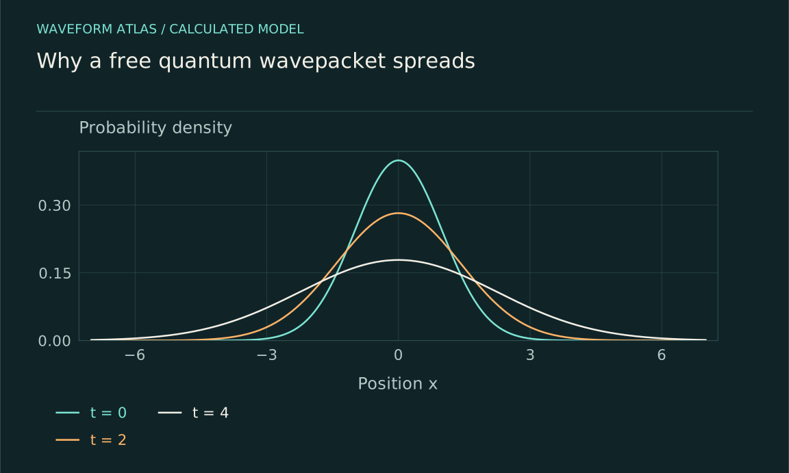
For an uncorrelated minimum-uncertainty Gaussian, Cov(x,p)=0 and σₚ=ℏ/(2σ₀). Substitution gives σₓ(t)=σ₀√[1+(t/t₀)²], with t₀=2mσ₀²/ℏ. The formula is not a universal width law for every quantum state. It is a particular result under specified assumptions. A state with a negative initial covariance can initially contract before expanding. A non-Gaussian state can develop a more complicated shape even though the general variance relation remains valid whenever the relevant moments exist.

This is an explicit moment calculation: insert x(t)=x+pt/m into the centred second moment and retain the symmetrized cross term. It extends the expectation-value method in Lecture 8; Lecture 7 supplies the free-Gaussian evolution, rather than stating this general covariance identity.

A dimensionless example makes the scale visible

Choose an illustrative Gaussian with σ₀=1 in a chosen length unit, and measure time in units of t₀. At t=0 the width is one. At t=t₀ it is √2, approximately 1.414. At t=3t₀ it is √10, approximately 3.162. The peak probability density falls inversely with the width, while the area under the density remains one. These are model calculations, not a set of measured data points.

The characteristic time grows with mass and with the square of initial width. Doubling the mass doubles t₀. Doubling σ₀ multiplies t₀ by four. Thus an initially broader minimum-uncertainty packet spreads more slowly in relative terms because its momentum spread is smaller. This counterintuitive feature is an excellent check on a simulation. If a program predicts the opposite while claiming these assumptions, inspect its width convention, units and normalization before interpreting the graph. A visible expansion rate only becomes meaningful after the preparation parameters are specified.

Correlation explains an increasing uncertainty product

As the packet evolves, momentum remains constant while position becomes correlated with momentum. Components associated with larger forward momentum contribute farther along the direction of motion. In phase-space language, the uncertainty distribution shears. Its projection onto the position axis broadens even though the full transformation preserves the state's information. The product σₓσₚ consequently increases from its initial minimum value.

This does not violate uncertainty relations or imply that the state has become mixed. For a Gaussian state the covariance-aware uncertainty condition includes both the product of variances and the covariance. The determinant of the covariance matrix remains constant under the ideal free shear. Looking only at the product of marginal widths discards that correlation. This distinction becomes experimentally important when a focusing operation later compensates the shear. A broad distribution can contain a predictable phase pattern that allows refocusing; a visually similar incoherent mixture may respond differently to the same control sequence.

Purity and a broad density are different questions

A pure state can have a wide spatial probability distribution. Purity concerns whether the complete state is described by one coherent amplitude or by a statistical mixture, not whether its density has a sharp peak. Under the free Hamiltonian, a pure initial state remains pure. The off-diagonal structure of its density operator changes in a representation-dependent way, but unitary evolution does not reduce its purity.

An ensemble with randomly displaced preparation centres can produce a broad average image too. So can a mixture of momentum kicks or a detector with poor spatial resolution. These cases can share similar densities while differing in correlations and phase-sensitive responses. A density image is therefore one observable among several. Use a phase-controlled reference, a refocusing sequence, or a validated tomography protocol when the question concerns coherence. No single test reconstructs every property without assumptions, so the report should identify the tested subspace and the detection efficiencies rather than attaching an unlimited claim to one recovered fringe.

Free evolution is reversible in the equations

The inverse of free evolution is mathematically U(−t), the adjoint of U(t). That statement concerns the structure of the model, not an instruction to make laboratory clocks run backward. Physical reversal generally requires a sequence of controls that implements an equivalent transformation on the relevant state. A lens-like phase operation, trapping sequence or interferometric protocol may compensate particular correlations without realizing a universal reversal of all dynamics.

This distinction prevents two opposite mistakes. A practical inability to refocus a packet does not prove that free spreading was fundamentally irreversible. Conversely, a successful refocusing operation does not mean every environmental interaction has been undone. The experiment demonstrates recovery under the measured preparation and control conditions. Its value comes from matching a specific prediction. A useful report compares the recovered width, phase response and probability with a calibrated baseline, and then varies the flight time or focusing strength to test the model over more than one convenient setting.

Detector resolution belongs in the model

A measured image is the state distribution filtered by the instrument. For approximately Gaussian independent broadening contributions, a simple model is σ_measured²=σ_packet²+σ_resolution². Timing jitter, initial position jitter and magnification uncertainty may add further contributions. The formula itself requires the assumed response functions; it is not a substitute for calibration. A fixed detector blur can obscure early spreading and make a later increase look like a sharp onset.

Estimate the instrument response with a source or reference whose size is independently constrained. Repeat the measurement at more than one magnification if possible. Fit the complete time dependence rather than comparing just two images. A genuine free-packet width curve has a characteristic mass and initial-width scaling. A fixed optical blur or timing error follows a different dependence. These controls improve the ability to detect small departures and prevent a visually dramatic broadening sequence from carrying more theoretical weight than its uncertainties support.

Use spreading as a baseline for new claims

A proposed stretching-induced reduction mechanism must predict something beyond the unitary broadening just described. It might alter an interference visibility, add diffusion, change a covariance relation or impose a dependence on a specified geometric variable. The proposal should identify that additional observable and its magnitude before the experiment. Otherwise, ordinary spreading can be mislabeled as evidence simply because the final density looks less localized.

A useful comparison measures both density evolution and a phase-sensitive quantity across a controlled sweep. Include an environmental model, calibration uncertainties and the probability of any postselected events. If the baseline works, the result is still informative: it defines a regime of reliable coherent transport. If it fails, the residuals guide the next experiment. The purpose of a free-packet model is therefore neither to dismiss geometric ideas nor to endorse them. It is to supply the quantitative reference that makes a claim about geometry experimentally distinguishable.

A useful dimensional check is that ℏt/(mσ₀²) is dimensionless: ℏ has units of mass times length squared divided by time. This catches missing powers of width before numerical results are interpreted.

Go to the original work.

These links identify the sources behind specific claims. Verification scope varies by source and is stated below.

1. 1 / University teachingZwiebach, Quantum Physics I, Lecture 7: Wavepackets and uncertainty ↗

   Barton Zwiebach (2016). 8.04 Lecture Note 7. https://ocw.mit.edu/courses/8-04-quantum-physics-i-spring-2016/6ca5bd79a2121967796f7c0b8f6f48c9_MIT8_04S16_LecNotes7.pdf

   Fourier representation and unitary free-particle spreading; equations are used as standard fundamentals, with original worked examples.

   Verification scope: MIT lecture PDF text inspected; not a claim of experimental evidence.

2. 2 / University teachingZwiebach, MIT 8.04 Lecture 8: Time dependence of expectation values ↗

   Barton Zwiebach (2016). 8.04 Lecture Note 8. https://ocw.mit.edu/courses/8-04-quantum-physics-i-spring-2016/72de1b688f3f40e1c42b26b3da29585a_MIT8_04S16_LecNotes8.pdf

   Section 3, Eq. (3.37), gives the commutator contribution for an observable with no explicit time dependence. The article explicitly derives any added time-derivative term.

   Verification scope: Section 3 read; the notes explicitly restrict their derivation to time-independent observables.