Fit a lifetime without hiding backgrounds or dead time

Define the parameter and the event

Before fitting, state what lifetime is being estimated. Is it excited-state population relaxation, particle survival, excess energy or a field-amplitude envelope? Define the preparation event and the event that ends survival. A detected photon can represent only one decay channel, while a missed click can mean either survival or an undetected event. The likelihood must reflect the actual relationship between physical events and recorded data.

Also identify the time variable: laboratory delay, reconstructed proper time or elapsed time since a herald. A constant clock-scale error rescales the inferred lifetime, while uncertainty in the start event can broaden or shift the distribution. These effects belong in calibration. A numerical fit cannot compensate for an undefined physical time origin simply by returning many significant figures.

Start with the ideal unbinned likelihood

For independent, complete exponential event times ti ≥ 0 with mean τ, the density is exp(−ti/τ)/τ. The likelihood is the product over events, so log L = −N logτ − Σti/τ plus constants. Differentiating gives the maximum-likelihood estimate τhat = Σti/N. The sample mean is therefore appropriate for this ideal dataset because the model and selection assumptions make it so.

The standard error is approximately τ/√N for a large sample, since the exponential distribution has variance τ². This uncertainty describes repeated samples under the model, not the spread of individual event times. The simple estimator is no longer generally correct when the data are truncated, background-contaminated or convolved with substantial timing response. Those features must be added before using the mean as a physical lifetime.

Include censoring rather than discard survivors

If some preparations survive until observation ends, their information is that the event time exceeds the cutoff. They are right-censored observations. Their likelihood contribution is the survival probability at that cutoff, not an event density and not zero information. For a constant-rate model with r observed events and total time at risk X, the rate estimate is r/X under the stated censoring assumptions.

Total time at risk includes the observed event times and the durations for which censored preparations were monitored. Ignoring the latter preferentially retains early events and can bias a naive mean downward. The statistical logic is general even though NIST’s handbook presents it in a reliability setting. The quantum or particle interpretation supplies the physical event model; the censoring calculation supplies the correct use of incomplete timing records.

Truncation requires parameter-dependent normalization

A sample containing only events inside a chosen window differs from a dataset that also records how many preparations survived beyond it. For accepted times between zero and T, an ideal truncated exponential density is exp(−t/τ)/[τ(1−exp(−T/τ))]. The denominator depends on τ and cannot be dropped from the likelihood. It accounts for the fact that the probability of entering the sample changes with the lifetime.

More complicated acceptance functions require a corresponding normalization integral. If efficiency varies with time or displacement, include that variation in the event model. The fitted distribution should integrate to one over the accepted sample when a conditional likelihood is used. Alternatively, an extended likelihood can include the expected event count. The choice must match what information was recorded, not whichever fit is easiest to draw.

Model preparation and timing response

A finite preparation pulse and detector jitter blur the physical time distribution. The recorded signal can be modeled as a convolution of the underlying decay with a measured instrument response, plus background. If the response width is comparable with the lifetime, fitting an unconvolved exponential near the peak can be strongly biased. A reference measurement with a sufficiently short known process can characterize the response under matched conditions.

The response can have asymmetry or long tails, not merely Gaussian jitter. Electronics, afterpulsing and delayed detection can create features that resemble slow emission. Calibration should therefore cover the range relevant to the claimed decay, including the tail if long-time deviations are the target. A single quoted timing resolution does not fully describe a response function that shapes the observed histogram.

Use the appropriate count statistics

For binned event counts, a Poisson likelihood is often appropriate when counts arise independently with predicted means per bin. Integrate the signal model over each bin rather than evaluating it only at the center when bins are not negligible compared with the timescale. Empty bins contain information and should not be discarded merely because their logarithm is undefined.

Fitting a straight line to logarithms can distort the error model, particularly at low counts or after background subtraction. An unbinned likelihood preserves timing information when individual events are available, while a well-designed binned analysis can still be effective. The method should be chosen for the data and model. The quality of a fit is judged through predictive checks and residuals, not through how straight the transformed plot appears.

Treat backgrounds as measured nuisance contributions

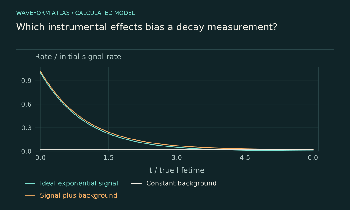
A constant background adds a floor that can flatten a decay tail. Time-dependent background, scattered excitation or delayed fluorescence can be more complicated. Measure controls under conditions that isolate plausible contributions, and propagate their uncertainty. Subtracting a best-estimate background and then treating the result as noise-free can underestimate uncertainty or create negative bins that are mishandled.

Varying source intensity and repetition rate can distinguish signal scaling from some background mechanisms. Spectral information may separate an unwanted channel. The background model should be physically justified and checked on control data rather than made arbitrarily flexible to improve a desired fit. When the late-time signal is small, uncertainty in the background can dominate even if the total experiment contains many events.

Check dead time and pile-up through rate changes

After an event, a detector may be temporarily unable to register another. Closely spaced pulses can merge or be assigned incorrectly. These dead-time and pile-up effects change the distribution in a rate-dependent way. In some time-correlated systems that retain only an early event per excitation cycle, later photons are underrepresented. Other detector models suppress high-rate portions differently. The actual electronics determine the bias.

A practical control reduces the source rate and checks whether the inferred lifetime converges while the preparation remains otherwise comparable. Independent detector calibration can constrain the response model. Do not apply one universal dead-time correction to every time-varying trace; formulas derived for steady Poisson rates have assumptions. Report the count regime and demonstrate that residual rate-dependent effects are below the claimed uncertainty.

Test model adequacy and uncertainty

Inspect residuals, vary reasonable fit boundaries and compare physically motivated alternatives such as one versus several populations. A fitted parameter that shifts beyond its reported uncertainty when the start time changes may indicate response or background problems. Interleave settings to expose drift. Separate statistical uncertainty from calibration and model uncertainty when they have different behavior under additional data collection.

Simulation can check whether the analysis recovers known parameters from data generated with the calibrated response and selection. Such a test validates the inference pipeline under that model, not the model’s completeness. A held-out reference preparation or independent detector provides a stronger external check. The final uncertainty should reflect the important assumptions rather than only the curvature of one convenient likelihood maximum.

Report enough information to reproduce the inference

State the fitted quantity, preparation, time origin, accepted events, censoring, response function, background and likelihood. Give the fit range, parameter correlations and uncertainty convention. Preserve raw timing or count data and calibration records where practical. If no events are observed, report a model-dependent limit rather than declaring an infinite lifetime or zero rate without qualification.

A lifetime is a compact summary of a physical model connected to a measurement process. The best fit is therefore not simply the smoothest exponential or the smallest formal error bar. It is the estimate that survives detector checks, selection accounting and alternative-model tests at the precision claimed. With those pieces explicit, the number can be compared across apparatus and used to test dynamics rather than merely describe a plotted slope.

A censoring example shows how much information can be lost by discarding unfinished trials. Suppose one hundred independent preparations are monitored for up to five microseconds. Sixty events occur, with their recorded event times summing to 120 microseconds; forty preparations survive to the cutoff. The total time at risk is 120+40×5 = 320 microseconds. Under the ideal constant-rate model, the rate estimate is 60/320 = 0.1875 per microsecond, corresponding to a mean lifetime of about 5.33 microseconds.

Taking the average of the sixty observed event times alone gives two microseconds, a very different and biased answer for this censored experiment. The missing trials are not failures of data collection: their survival to five microseconds is informative. This arithmetic assumes perfect event detection, a common preparation and no background. If those assumptions fail, the likelihood must change rather than applying the formula mechanically. The example also explains why the full attempt count and stopping rule should be retained with the event list. A histogram of successful detections alone may no longer contain enough information to reconstruct the intended lifetime without additional assumptions.

Go to the original work.

These links identify the sources behind specific claims. Verification scope varies by source and is stated below.

1. 1 / Official researchParticle Data Group (2024), Statistics review by G. Cowan ↗

   Likelihood construction, parameter-dependent normalization, uncertainty and inference for event data.

   Verification scope: Official review PDF sections on likelihood, sample means and parameter estimation inspected; examples below independently derived.

2. 2 / Official researchNIST/SEMATECH e-Handbook, Maximum likelihood estimation for censored lifetime data ↗

   Exponential likelihood with censored observations and total-time-at-risk estimator.

   Verification scope: Official handbook page and displayed likelihood derivation inspected.

3. 3 / Primary experimentWare et al. (2007), Calibrating Photon-Counting Detectors to High Accuracy: Background and Deadtime Issues ↗

   Detector calibration issues involving background, dead time, pulse timing and afterpulsing.

   Verification scope: Official NIST publication abstract and bibliographic record inspected; not a full detector-paper audit.