The environment can change a decay rate

The surroundings are part of the transition

An emitter does not radiate into an abstract empty destination. It couples to electromagnetic modes determined by its surroundings. A cavity, interface or photonic structure changes those modes and their local field strengths. The transition rate can therefore depend on where the emitter sits, how its dipole is oriented and how its frequency aligns with the structure. The environment is part of the physical system setting the emission dynamics.

This does not mean that an external observer chooses a lifetime by watching the emitter. It means that changing the Hamiltonian and available final states changes the transition probability. The distinction is important for interpreting a longer or shorter decay trace. A controlled environmental intervention is a conventional physical mechanism, not evidence that the passage of time itself became more or less destructive.

Connect coupling and mode density

In a weak-coupling continuum approximation, a rate can be expressed through a transition matrix element and the density of available final states. Both ingredients matter. Increasing the number of modes near a transition can increase emission only to the extent that the emitter couples to them. A field node or an unfavorable dipole orientation can suppress coupling even in a structure with a strong resonance elsewhere.

The relevant optical quantity is often a local and polarization-sensitive mode density rather than a simple count of modes in the whole device. A complete calculation uses the actual geometry and material response. The intuitive statement that more available modes gives faster emission is useful, but it is not a substitute for evaluating the coupling at the emitter’s position and frequency. Lossy or dispersive materials can require a more careful electromagnetic treatment.

State the ideal Purcell scale

For a resonant, well-aligned dipole in a suitable weak-coupling single-mode cavity model, the familiar enhancement scale is F_P = [3/(4π²)](λ/n)³Q/V. Here Q is the cavity quality factor and V an appropriately normalized mode volume. The formula’s assumptions include spectral and spatial overlap, a suitable dipole orientation and a regime where a rate description remains meaningful. Different definitions of the background rate must also be handled consistently.

As an arithmetic illustration, take Q = 1,000 and V = 10(λ/n)³. The ideal scale is about 7.60. This is not a guaranteed total decay enhancement for a real emitter. Background channels, detuning, dephasing and nonradiative loss can change the observed result. The formula is most useful as a design estimate whose assumptions are checked, rather than a promise based only on a large quoted Q.

Detuning and bandwidth limit enhancement

A cavity resonance affects emission most strongly when the emitter and mode overlap spectrally. If the emitter is detuned or its line is much broader than the cavity response, the effective enhancement can be reduced. Spectral diffusion can make that overlap fluctuate between trials. A lifetime measured over many trials may then reflect an average over changing conditions rather than one fixed rate.

A useful experiment scans detuning and compares the rate with the predicted spectral response. It also characterizes the emitter’s linewidth and the cavity’s loss channels. A larger Q narrows the cavity resonance, which can improve an ideal on-resonance scale while making alignment more demanding. The tradeoff should be analyzed for the actual emitter and task. A narrow resonance is not automatically the best source of usable photons under every noise condition.

Suppression is as informative as enhancement

Photonic structures can reduce the available radiative channels in a frequency range or redirect emission away from selected modes. Lodahl and colleagues demonstrated controlled changes, including inhibited and enhanced spontaneous-emission dynamics, in quantum dots embedded in photonic crystals. The result is a concrete example of environment-dependent rates in a specified material and geometry.

Suppression of one channel does not guarantee an indefinitely stable excitation. Other radiative modes, leakage, material absorption and nonradiative processes can remain. A finite structure also differs from an ideal infinite band-gap model. The measured lifetime should therefore be compared with the total channel budget. A weak detected signal may indicate inhibition, but it may also indicate that emission was redirected or collection became inefficient. Additional measurements are needed to distinguish these possibilities.

Separate lifetime from quantum yield

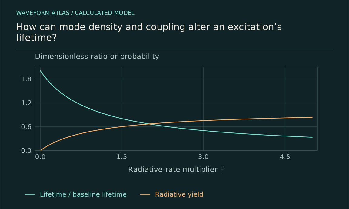
Let Γrad and Γnr be radiative and nonradiative rates in a simple model. The lifetime is 1/(Γrad+Γnr), while the radiative yield is Γrad/(Γrad+Γnr). Increasing the radiative rate can shorten the lifetime while increasing the fraction of excitations that produce photons. Increasing the nonradiative rate can also shorten the lifetime, but reduces that fraction. The same direction of lifetime change can therefore correspond to opposite changes in useful emission.

For a hypothetical emitter with both rates equal to 10⁷ per second, the lifetime is 50 nanoseconds and yield one half. Increasing only Γrad fourfold gives a lifetime of 20 nanoseconds and yield 0.8. These numbers expose the need to measure more than a decay constant. A faster emitter is not automatically a brighter or more efficient source unless the altered channels and collection are known.

Collection efficiency is another independent factor

A structure can redirect radiation into a detector without changing the total decay rate much. Conversely, it can enhance total emission into modes the detector poorly collects. The detected photon probability is the radiative yield multiplied by the relevant collection and detection efficiencies, with additional spectral or temporal selection if applied. Brightness therefore combines source preparation, physical channels and optics.

A useful characterization reports lifetime, detected counts per preparation and collection assumptions separately. Calibration across wavelength and polarization is important when the structure changes the output spectrum. Comparing only raw count rates can mistake improved collection for a Purcell enhancement or mistake reduced collection for inhibited emission. The physical rate inference should be supported by time-resolved and spectral evidence, not by brightness alone.

Strong coupling requires a different dynamical picture

If coherent emitter–cavity exchange becomes faster than the relevant losses, excitation can oscillate between the two systems. The cavity is then not merely a memoryless destination characterized by one enhanced decay rate. The combined state and its losses must be modeled. Damped oscillations, split resonances or multiple timescales can arise depending on the preparation and measurement.

This is one reason a weak-coupling enhancement formula cannot be extrapolated indefinitely. Changing Q or mode volume can move the system into another regime. The theory should compare coupling strength, detuning and linewidths before selecting a rate equation. A measured nonexponential trace in this setting may be exactly what standard coupled dynamics predicts, rather than evidence that the notion of decay has failed or that a new collapse law is required.

Other environmental changes can confound the comparison

Placing an emitter near a structure can alter temperature, charge noise, chemical conditions or nonradiative coupling as well as the optical mode density. These changes can affect both lifetime and coherence. A controlled comparison should identify which intervention is intended and monitor plausible accompanying effects. Otherwise a rate change may be attributed to the cavity when another environmental channel dominates.

Detuning scans, spatial controls and reference emitters can help, but each needs a model of what remains fixed. A reference located elsewhere may experience different material conditions. A temperature change may shift both the emitter and cavity. The strongest inference uses several observables and controls whose predicted dependencies distinguish the competing explanations. The goal is a causal account of the rate change, not merely a before-and-after difference.

Engineer the environment for a defined task

A useful design begins with the desired outcome: faster emission, longer storage, higher radiative yield, better collection or preserved coherence. These goals can conflict. The relevant model includes the emitter, mode structure, losses, detuning, noise and detector. It predicts the quantity the task actually needs rather than treating one nominal enhancement factor as a universal performance score.

Environment control demonstrates that a lifetime is a property of a preparation and its physical couplings. It can be changed through a measurable intervention without invoking an observer-dependent clock or an unexplained disappearance. By separating total rate, radiative fraction, output direction and detection efficiency, an experiment can show exactly what was improved or suppressed and where the excitation’s energy ultimately went.

Suppression of radiation gives a complementary numerical example. Begin with Γrad = Γnr = 10⁷ per second, so the total lifetime is 50 nanoseconds and radiative yield is one half. Reduce only the radiative rate to one quarter of its original value. The total rate becomes 1.25×10⁷ per second, giving a lifetime of 80 nanoseconds, while the radiative yield falls to 0.2. The excitation lasts longer but is less likely to produce a useful photon.

The inverse radiative rate alone is now 400 nanoseconds, which is not the measured total population lifetime because the nonradiative channel remains. If that channel were negligible instead, suppressing radiation would lengthen the total lifetime while leaving the eventual radiative yield near one. These different outcomes show why a rate budget is necessary. A lifetime and a brightness measurement together can help identify which channel changed, provided collection is independently calibrated. The intervention should also be checked for added absorption or charge noise, since a structure intended to inhibit radiation can introduce another loss mechanism and reverse the expected benefit.

Go to the original work.

These links identify the sources behind specific claims. Verification scope varies by source and is stated below.

1. 1 / Primary experimentLodahl et al. (2004), Controlling the dynamics of spontaneous emission from quantum dots by photonic crystals ↗

   Enhanced and inhibited emission rates in the specified photonic-crystal quantum-dot system.

   Verification scope: Publisher abstract and relevant displayed passages inspected; not a claim of independent replication or full-paper audit.

2. 2 / Primary theoryNoda, Fujita and Asano (2007), Spontaneous-emission control by photonic crystals and nanocavities ↗

   Research-authored explanation of optical mode engineering, emission suppression and cavity enhancement.

   Verification scope: Primary publisher abstract inspected; idealized equations are separately identified as models.

3. 3 / University teachingPreskill, Quantum Information, Chapter 3: Measurement and Evolution ↗

   Measurement operators, channels, dephasing, amplitude damping and open-system evolution.

   Verification scope: Author-hosted lecture PDF inspected for relevant sections; not an exhaustive audit of every lecture derivation.