Read a constant-rate decay law
Adjust the controls, inspect the calculated response and use the reading links to place the model in its physical context.
Interactive model: Read a constant-rate decay law. Enable JavaScript to adjust its controls.
S(t) = exp(−t/τ); t½ = τ ln 2
Memoryless exponential survival model; time and lifetime use the same arbitrary unit. Expected survivors are calculated for an initial population of 1,000. Real quantum survival can depart from this law at short and long times.
What this model assumes
Memoryless exponential survival model; time and lifetime use the same arbitrary unit. Expected survivors are calculated for an initial population of 1,000. Real quantum survival can depart from this law at short and long times.
How to explore it
Begin with the default values. Change one control at a time and watch both the graph and the readouts. Then reset the model and change another parameter. This isolates which input produces the effect you are seeing.
The plotted values are generated from the displayed equation. Downloading the calculated data lets you inspect the numerical series or compare it with a calculation of your own. The data are synthetic model outputs, not observations from an apparatus.
Before carrying a prediction into an experiment, match the model’s assumptions to the actual system: the relevant degrees of freedom, boundary conditions, noise, losses and measurement convention. The linked articles explain which comparison is physically meaningful.
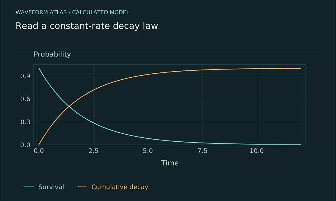
Calculated model curves. Memoryless exponential survival model; time and lifetime use the same arbitrary unit. Expected survivors are calculated for an initial population of 1,000. Real quantum survival can depart from this law at short and long times. Default control values are used in this fixed figure.
Download SVG ↓Decay and relaxation
What is decaying?
Does decay refer to amplitude, energy, excited-state population, coherence, or particle survival?
When exponential decay is a useful approximation
Which assumptions produce a constant decay rate?
Two decay constants can describe the same oscillator
Why do amplitude and stored energy fall at different exponential rates?
An excited atom transfers energy into the field
How does a radiative transition change the atom-plus-field system?
An unstable particle and its products
How do conservation laws constrain a decay channel?
Losing energy and losing phase memory
What distinguishes population relaxation from dephasing?
The environment can change a decay rate
How can mode density and coupling alter an excitation’s lifetime?
What changes at very short or long times?
Where can simple exponential fits fail, and what evidence is needed?
Fit a lifetime without hiding backgrounds or dead time
Which instrumental effects bias a decay measurement?
Decay products do not establish a new collapse law
How does tracing the full system change the interpretation of a disappearing excitation?